Neural Network with cWB
How to make and use Artificial Neural Networks (ANNs)
| Introduction: | |
| What are ANN: | Artificial Neural Networks |
From cWB output to ANN creation
| TF selection: | extract the TF representation of the events from cWB 2G analysis; |
| Matrix Conversion: | convert the TF representation of each event in a NDIM \times NDIM matrix; |
| Information collection: | save all the useful information in a root-file; |
ANN creation and usage
| ANN Creation: | tools for the ANNs creation; |
| ANN Use: | tool for the ANN applications on different data sets; |
| ANN Average: | tool for the application on different data sets of more ANNs (averaging their outputs); |
| ANN Tests: | tools for deeper analysis; |
Vinciguerra_2014_MasterThesis.pdf.Introduction
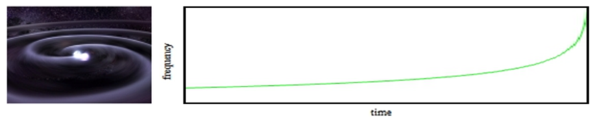 |
| *Compact binary coalescence: an example of interesting gravitationa wave source and its typical emission in the TF plane.* |
What are ANN
- neuron definitions: neurons are characterized by a threshold, which is generally treated as a surplus weight with default input equal to -1, and by an activation function which collectd all the neuron inputs to return an output. Different function can be used to define the neurons and the sigmoid functions are the most common.
- connection properties:
- feedback networks: the connections can have both the direction or anyway some neurons comunicate toward the inputs;
- feedforward networks: the connections have only one direction.
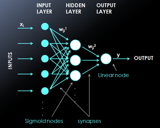
WHAT ARE MULTI-LAYER-PERCEPRTONs?
Multi Layer Perceptrons a particular feedforward ANNs where the neurons are organized in groups called layers. There are no connection between neurons belonging to the same layer. There exist three typs of layers:
- input layer: its task is to define the input quantities and pass them to the successive layer. The neurons belonging to this layer are said inactive because their transfer function is 1;
- hidden layers: each neurons of these layers calculates the weightened sum of its inputs and the correspondent output through the activation function. The inputs of such calculation units are the output quantities of the neurons bolonging to the previous layer. The user can use how many hidden layers he desires;
- output layer: the neurons belonging to this group act on their inputs as the ones which define the hidden layers. Their output values should be similar to the desired ones, according to the belonging class of events. This result can be reached with an appropriate training procedure.</li>
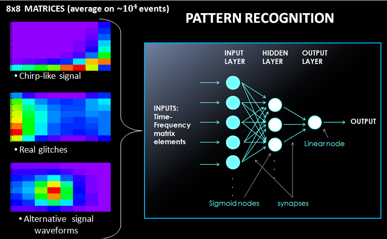
ANN architecture
- Input layer: it is constituted by neurons. The input quantities are the values of the normalized-likelihood calculated for each TF interval in the matrxi conversion step. Each elements of the resulted frame correspond to an ANN input neurons.
- Hidden layer: the number of these layers and the one of their neurons are free. The neurons are define by a sigmoidal activation function.
- Output layer: a single neuron, characterized by a linear activation function, is used to provide the final output value. The chosen choice is to train ANNs with desired output 1 for events belonging from the targer class, 0 otherwise.
TF selection
The plugin is a C++ function which is called by the pipeline different stages of the analysis and can be used to customize the analysis (see Plugins)
MAIN CHARACTERISTICS
- Main task:
- extract information about the TF representation of the events. The cWB 2G analysis is based on the TF decomposition of the signals through the Wilson-Daubechies-Meyer (WDM) TF transformation in different TF resolutions (levels). The analyzed levels are chosen by the users in the user_parameters.C file. The final event recostruction in the TF plane is given by a collage of the most energetic pixels in the different levels. To male this representation complete and independent when a pixel is selected its contribute is removed by the other levels using appropriate tables.
- Information saved:
- a complete and independent representation of the event composed by selected pixels bolonging to different TF levels.
- Plugin type:
- CWB_PLUGIN_OLIKELIHOOD.
- Extra information:
- it can be used also to enable event monster plots and to introduce simulated noise and waveforms. To perform these addictional tasks the code uses different plugin types, acting in different moments of the cWB 2G analysis.
To extract the necessary information from the 2G analysis you need to have in the “macro” directory of the simulation the following files:
- CWB_Plugin_NN.C strictly necessary for the information extraction;
- CWB_Plugin_NN_Config.C or CWB_Plugin_BRST_Config.C these files or similar ones are used to define the parameters of the waveforms you are interested in.
plugin=TMacro("macro/CWB_Plugin_NN.C");
plugin.SetTitle("macro/CWB_Plugin_NN_C.so")
configPlugin=TMacro("macro/CWB_Plugin_NN_Config.C");
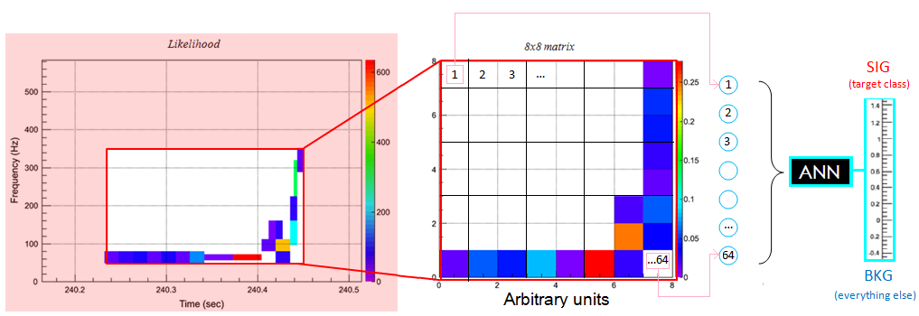
Matrix Conversion
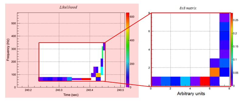
To use ANN for pattern recognition it is necessary to convert the TF representation of an event in a matrix whose elements constitute the ANN inputs. The algorithm implemented performs a conversion of the TF representation of the event in a square matrix.
Legend
|
Useful relations
|
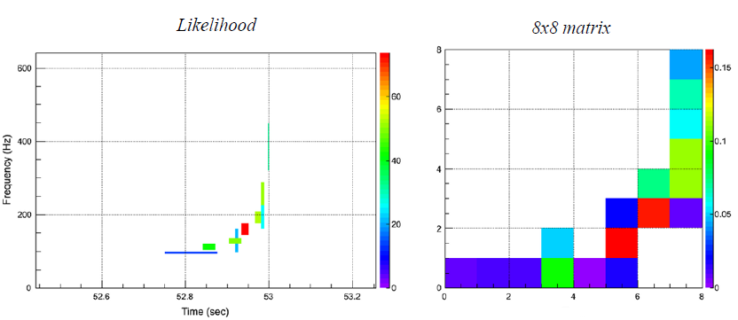
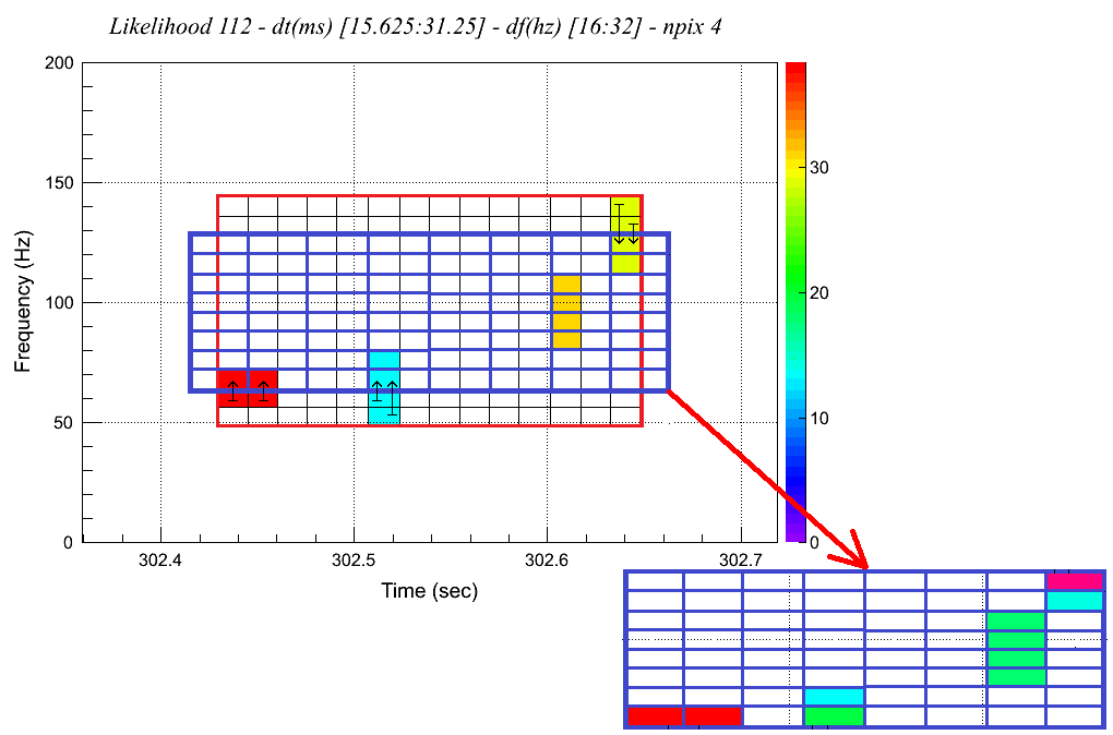
For each event, the TF representation is composed of pixels selected by cWB 2G. They are well defined in time and frequency: each of them belongs from a particular decomposition level characterized by fixed resolutions (\( T \)Therefore different levels can be involved. Unfortunalety the time and frequency resolutions are connected in every level by the relation: \( T \times \delta f=0.5 \)Each of these selected pixels is also characterized by a likelihood value different from zero. This is the key quantity which defines the ANN inputs. To use this information for the ANN training you can imagine the TF representation of an event as an image which will be treated in the following way.
How it works
- ZOOM:
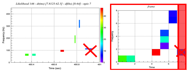
- PIXEL REMOVAL:
for the chirp recognition it is useful to remove some selected pixels if they satisfy determined conditions. Indeed if the analysis selects a noisy pixel after the chirping time it strongly modifies the resulted matrix and therefore comprimises the ANN performances. The process, by which the pixels are removed, is descrided in the following.
- The macro singularly considers the pixels according to the order of their central times starting from the last o>e. The pixel considered is removed if the cumulative likelihood is less than the 10\% of the one of the whole event. The cumulative likelihood is calculated summing the likelihood value of the considered pixel to the ones of the pixels just removed.
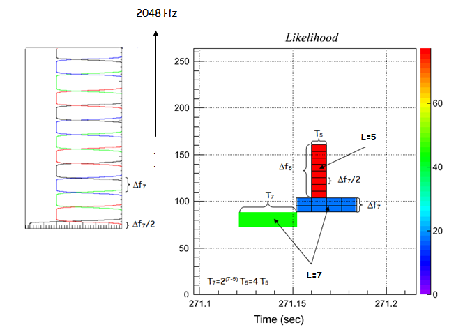
FRAGMENTATION IN FUNDAMENTAL UNITS:
individuation of the smallest resolutions, in time \( T_{min} \)frequency \( \delta f_{min} \)analysis. The best resolution are determined by the decomposition levels \( L \)during the analysis: \( T=2^L\cdot r_s^{-1} \)\( r_s \)MATRIX CREATION:
the image is converted in a matrix with the desired dimensions (\( DIM_T \)representation (the frequency one is treated at the same way), different processes can be adopted depending on the value of \( n_T=\Delta T\cdot (T_{min})^{-1} \)
- If \( n_T=l_T\cdot DIM_T \)
- else two procedures can be applied according to the value of \( d \)defined by the relation: \( (n_T+d)=l_T\cdot DIM_T \)
- if \( d<4 \)(increasing the \( T_f \)(decreasing the \(
- T_i \)starting from the right one: \( T_i=T_i-int(d/2)\cdot T_{min} \)\( T_f=T_f+[d-int(d/2)]\cdot T_{min} \)\( T_f-T_i=(T_f-T_i)+d\cdot T_{min}[d-int(d/2)]\cdot T_{min} \)
- else the macro remove the necessary \( DIM_T-d \)(because
- for our purpose of chirp beahviour recognition this is the less invasive choice). However the process consists also in adding the likelihood value of each removed pixel to the one associated to the first time-interval: \( T_i=T_i+(DIM_T-d)\cdot T_{min} \)\( T_f-T_i=(T_f-T_i)-(DIM_T-d)\cdot T_{min}[d-int(d/2)]\cdot T_{min} \)
- If \( n_{T(F)} < DIM_{T(F)} \)
Then the matrix and therefore the ANN inputs are defined in the following way: the fundamental units are divided in groups of \( l_T\times l_F \)likelihood values is calculated. This will be the ANN input value. Finally all the (\( DIM_T\times DIM_F \)
Usage
It requires as two strings as argument:
root -l -b 'ClusterToFrameNew01_dtmin_approx_cent.C+("in_path/in_file.root","out_path/out_file.root")'
The first has to be the name of the root file provided by the cWB 2G analysis (this means the name of a single job file or the name of the merge file), whereas the second has to be the desired name of the root output file.
This macro has no argument, but you have to fill it with the right data (directory containing the files to merge, output directory and label of the output file), following the instructions you can find opening it. The tree name is just rightly written.
root -l -b MergeTrees.C
Information collection
What is it
- the \( nIMP \)
- the matrix dimension (\( NDIM=DIM_T=DIM_F \)thought to convert the TF representation of the events in a square matrix;
- the classification tag. It is a integer variable, called “type” (see here), used to define the target class. It represents the desired output and in the implemented case and therefore it assumes the value of “1” when the events belongs to the target group, “0” otherwise.<
Further secondary information are saved; here is the list: the names of the two input files, the duration of the last 20 selected pixels, the duration of the event, its central frequency, its central time, the applied option on the amplitudes (explained in the following), an index, the event number of the belonging class and the event weight.
requires some arguments:
        root -l -b 'TreeTest_CTFmod.C+("SIG_merge.root","BKG_merge.root","nnTREE/out_file.root",0/1,NDIM,nINP)'

- **SIG_merge.root**: the path and the name of the file which
  contains the events belonging to the target class.
- **BKG_merge.root**: the path and the name of the file which
  contains the events belonging to the background group.
- **nnTREE/out_file.root**: the path and the desired name of the
  output file.
- **0/1**: it represents what was called applied "option on the
  amplitudes", indeed it describes the amplitudes treatment.

  -  Instead of *1* you can write any integer number, except *0*,
     obtaining the same results: the normal consideration of the
     selected pixel amplitudes. In this way the coordinate, that
     determines the ANN inputs, can assume a continue scale of value.
  -  However you can also adopt a different approach, choosing and
     writing as argument the number *0*. In this way the number
     associated to each matrix element (normalized-likelihood for fixed
     time and frequency intervals) becomes a binary variable, whose
     value is set to 0 if originally it was less than 0.001, to 1
     otherwise.

- The integer **NDIM**: this value represents the desired matrix
  dimension.

  The choice of \\( DIM = 8 \\)therefore it has been deeply
  investigated. Anyway remember that it must be chosen consistently
  with the matrix dimension used to convert the TF representation of
  the events.

- The integer **nIMP**: it represents the desired number of ANN
  inputs. Having implemented a conversion in a square matrix its value
  has to be \\( NDIM^2 \\). Obviously also in this case, it must be
  consistent with the choices defined in the previous steps.
NOTE: Some macros implemented for applications require this file to be in a directory whose name end with “nnTREE”, therefore you are invited to built such a directory and to save the output file there.
ANN Creation
Algorithm core: ROOT-toolkit TMultiLayerPerceptron for ANN creation.
| ANN creation-Equipment: | the particular enviroment which is necessary; |
| ANN creation-commands: | how to use the files and their required arguments. |
ANN creation-Equipment
To create ANNs with the cwbANN_purity_BoS.C or cwbANN_purity_SoB.C files some directories are required in the location where the command is used:
NN: this directory collects the output root files which contain the trained ANNs (one for each created ANN);
thresFiles: this directory collects files which contain some images and some data about the correctly and the wrongly classified events of the set provided for the training. To perform the count different thresolds on the ANN output are applied and the correspondent information is saved (one for each created ANN);
selectTREE: this directory collects the files associated to the events selected for the ANN training. They contains the main properties of the events used to train the ANN (one for each created ANN);
mlpa_canvas: this directory collects images (one for each created ANN) which represent some characteristics of the selected events.
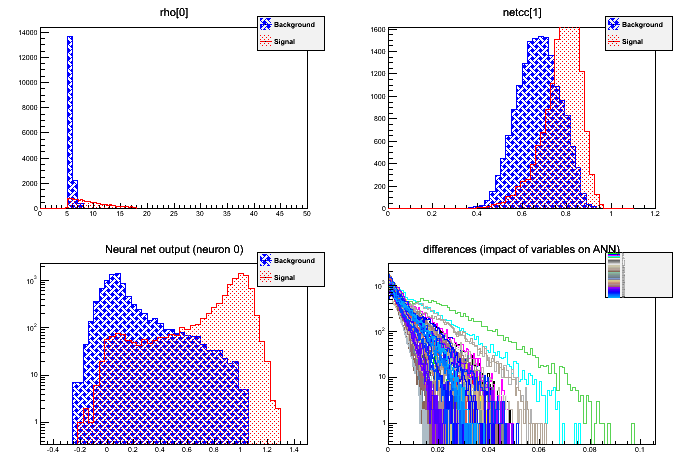
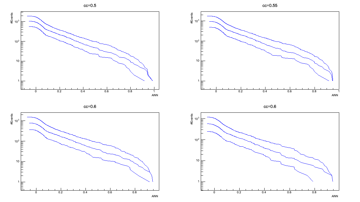
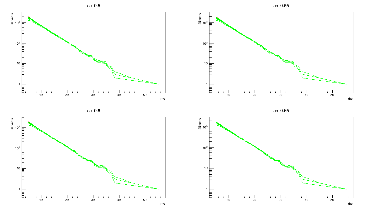
Each saved picture is composed of 4 graphs which have in ordinate the number of the events. The histrograms on the top analyse the whole set of events, while the bottom ones refers to exaples of the Test sample. Summarizing:
- top-left (whole selected set):ordinate = event cout, abscissa = cc (Network Correlation coefficient);
- top-right (whole selected set):ordinate = event cout, abscissa = rho (effective correlated SNR);
- bottom-left (Test sample):ordinate = event cout, abscissa = ANN output (red = SIG, blue =BKG);
- bottom-right (Test sample):ordinate = event cout, abscissa = difference in ANN output, varying each input (1 input = 1 color)
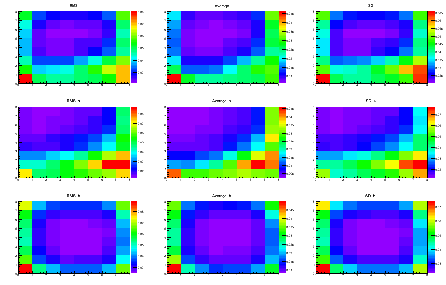
- PropertyGraphs: this directory collects images (one for each created ANN) which represent the mean values of each frame elements of the set of events selected for the ANN training. | The first row concerns the whole set of selected events, the second the SIG ones and the third the BKG ones. The first column represents the RMS of each pixels of the matrix, the second the average and the third the variance.
TRAIN_GRAPHS: this directory collects images (one for each created ANN) which contain 6 graphs (see the “LEGEND” table).
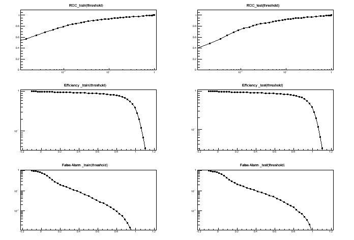
- top-left (Train sample):ordinate = True_Alarms/Total_SIG_events, abscissa = False_Alarms/Total_BKG_events;
- center-left (Train sample):ordinate = True_Alarms/Total_SIG_events, abscissa = threshold on ANN output;
- bottom-left (Train sample):ordinate = False_Alarms/Total_BKG_events, abscissa = threshold on ANN output;
- center-right (Test sample):ordinate = True_Alarms/Total_SIG_events, abscissa = False_Alarms/Total_BKG_events;
- top-right (Test sample):ordinate = True_Alarms/Total_SIG_events, abscissa = threshold on ANN output;>
- bottom-right (Test sample):ordinate = False_Alarms/Total_BKG_events, abscissa = threshold on ANN output;
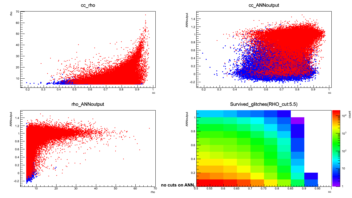
CC_OUT: this directory collects images (one for each created ANN) composed of 4 graphs. All the four pictures refer to the events of the Test sample. Three of them are scatter plots where the red-dots represent the <font color=”red”>SIG</font> events and the blue-points the <font color=”blue”>BKG</font> ones. The meaning of each graph is briefly explained in the following (see the “LEGEND” table):
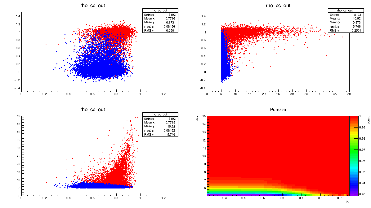
- top-left:ordinate = ANN output, abscissa = cc (Network Correlation Coefficient);
- top-right:ordinate = ANN output, abscissa = rho (Effective Correlated SNR);
- bottom-left:ordinate = rho (Effective Correlated SNR), abscissa = cc (Network Correlation Coefficient);
- bottom-right:ordinate = statistical purity (True_Alarms/[True_Alarms + False_Alarms]).
- ErrorGraphs:
- this directory collects images (one for each created ANN) where are represented the error-values (ordinate) in function of the epochs number.This kind of pictures are useful to choose the number of epochs which better satisfies the compromise between gain and time. Be careful: an exagerate number of epochs can provoke a lost of generality and the algorithm can be able to recognize only the examples analysed during the training procedure. |
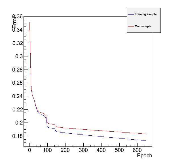 |The red-line refers to the Train sample, the blu-one to the Test sample. | |
LEGEND
Taget-Signal presence
Taget-Signal absence
Hypotesis of SIG presence
True Alarm
False Alarm
Hypotesis of SIG absence
False Dismissal
True Dismissal
The two files
or
which differ only in the superposition of the dots in all the scatter plots, can be found in the directory /home/waveburst/ANN/Summary/NNcreation, together with all the necessary directories. Here there are two addictional directories: the log and condor. These last are useful only if the ANN creations happen as jobs on clusters.
ANN creation-commands
file if you want to create an ANN emphatizing the BKG events in the output scatter plots (easier view of the False Alarms); | Use the
file if you want to create an ANN emphatizing the SIG events in the output scatter plots (easier view of the False Dismissals). | | The general command is:
root -l -b 'cwbANN_purity_BoS.C+(nTrainS, nTrainB, "architecture", "in_file.root", initial_SIG,
                                 initial_BKG, max_rho, max_cc, learning method, epochs)'
nTrainS: number of the examples belonging to the SIG class that will be used to train the ANN (whole set).
nTrainB: number of the examples belonging to the BKG class that will be used to train the ANN (whole set).
architecture: a string which defines the desired hidden layers, which are separated by colons, by fixing the number of their neurons. In this way the Multi-Layer-Perceptron architecture is determined, indeed the output and the input layers are fixed by the code and by the previous steps. Defined architecture:
- input layer with \( NDIM\times NDIM \)
- output layer with 1 output linearneuron.
- hidden layers with 3 hidden layers with respetively (from inputs to output): 16, 32 and 16 neurons.</li>
in_file.root: this argument must define input file which contains the events that you are going to use to train the ANN. This file must be built following the previous steps.
initial_SIG: this number establishes the first SIG-event selected to compose the Train and the Test samples. All the events in the input-file are tagged by an ordered increasing index, used to identify them. The other nTrainS-1 examples are selected from this starting point, following their order inside the input-file.
initial_BKG: this number establishes the first BKG-event selected to compose the Train and the Test samples.The other nTrainB-1 examples are selected from this starting point, following their order inside the input-file. Having saved in a single input-file all the events, starting from the SIG ones, the index of this first BKG event must be greater than the total number of the SIG signals.
max_rho: this argument defines the maximum rho (Effective Correlated SNR) represented in the purity-graph.
max_cc: this argument defines the maximum cc (Network Correlation Coefficient) represented in the purity-graph.
learning method: this parameter defines the learning method used to train the ANN. It is therefore an index which can take integer values in the interval [1,6]:
- Stochastic minimization
- Steepest descent with fixed step size (batch learning)
- Steepest descent algorithm
- Conjugate gradients with the Polak-Ribiere updating formula
- Conjugate gradients with the Fletcher-Reeves updating formula
- Broyden, Fletcher, Goldfard, Shanno (BFGS) method
To learn more about ANN learning methods visit the Wiki-page.
epochs: this argument determines the epoch number. This parameter fixes how many times the Train Set is considered before defining the final ANN structure, i.e. before fixing the weight and the threshold values.
You can find both the files in the /home/waveburst/ANN/Summary/NNcreation directory.
root -l -b 'cwbANN_purity_BoS.C+(16384,16384,"16:32:16","nnTREE/nnTree_CTF01_dtmin_app_cent_recSIG25_BKG.root",0,1200000,15,0.9,5,650)'root -l -b 'cwbANN_purity_SoB.C+(16384,16384,"16:32:16","nnTREE/nnTree_CTF01_dtmin_app_cent_recSIG25_BKG.root",0,1200000,15,0.9,5,650)'WARNING: the files used on the example are obtained by the last version of all the process, BUT the data were not correctly analysed in the cWB process. Thus don’t take care too much about the results.
ANN Use
| File for Test an ANN-Explanation: |
| File for Test an ANN-Use: |
File for Test an ANN-Explanation
- the ANN performances
- the impact of the ANN output on the event evaluation
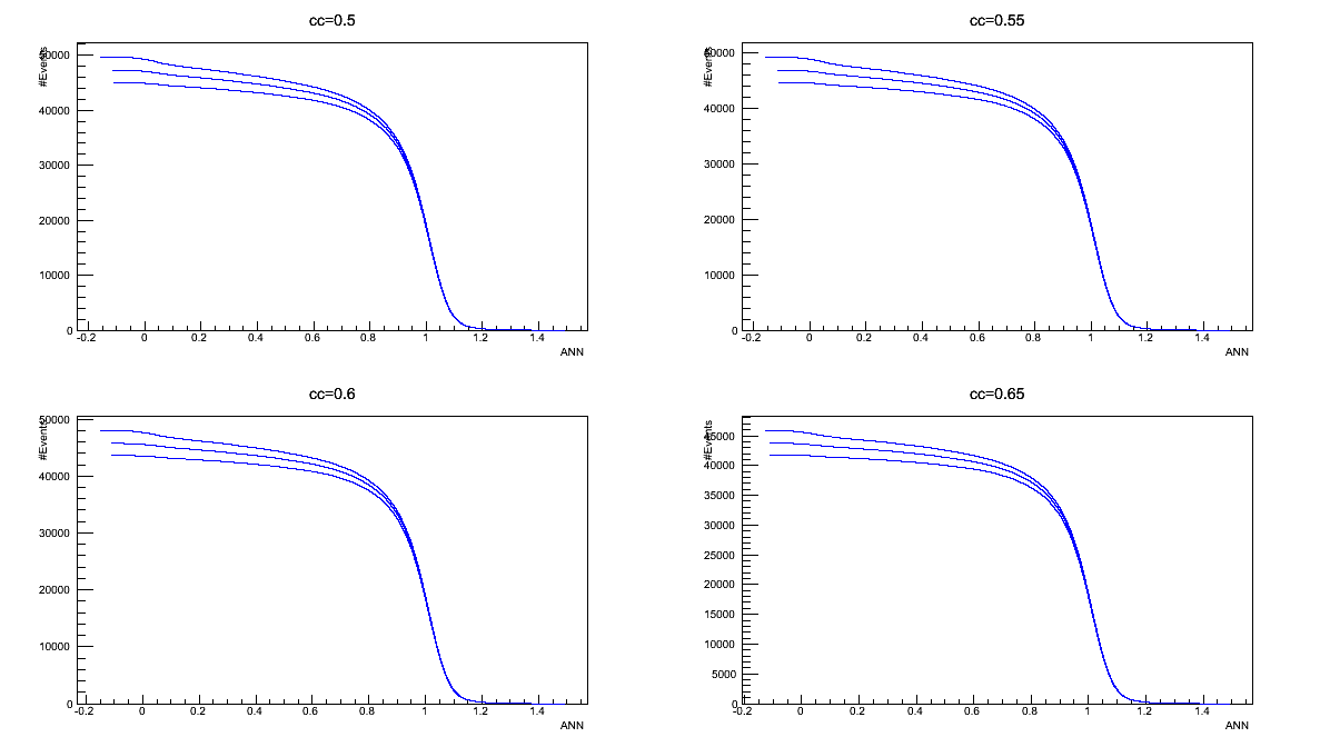
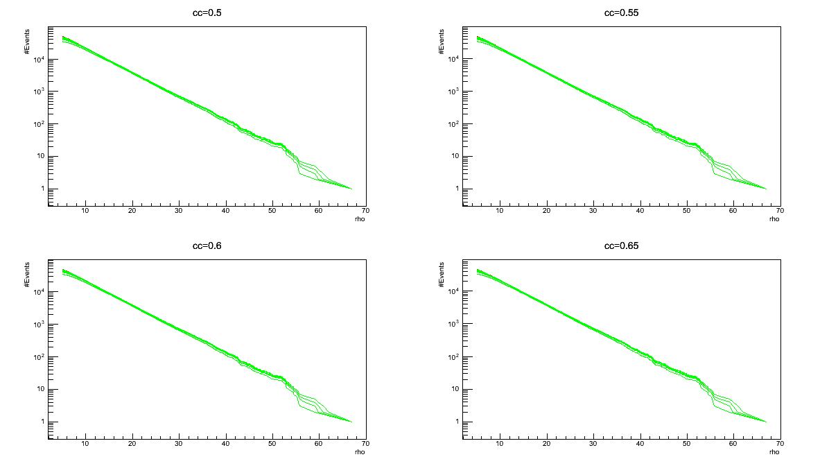
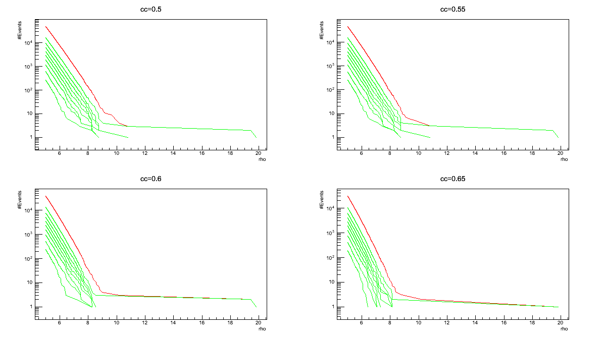
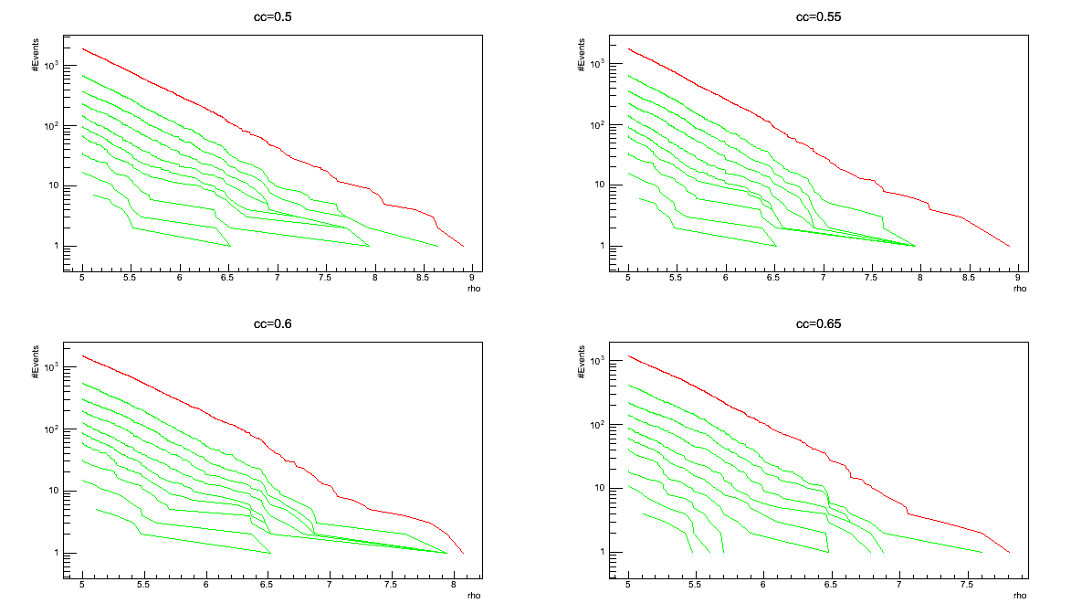
N_ANN_S_NN_*_FILE_*_dANN0*_uf*.png (only SIG events)
three different curves concern different thresholds on rho parameter: cc parameter: \( rho_{th}= \)survive the cuts and are taken into account in the graphs;
three different curves concern different thresholds on rho parameter: cc parameter: \( rho_{th}= \)survive the cuts and are taken into account in the graphs;
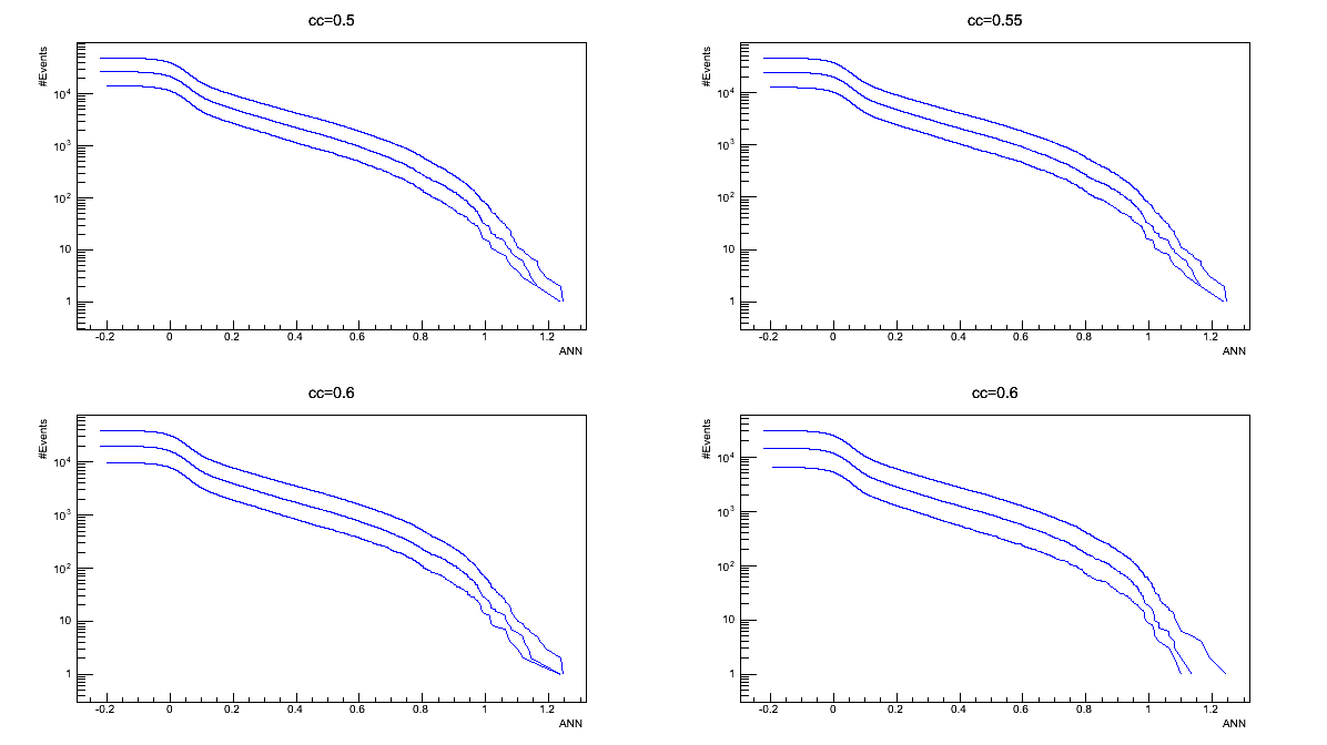
each graph contains ten different curves concerning different thresholds on ANN \ output parameter:
- to the red curve corresponds no cut on ANN \ output
- to the green curves correspond threshold values in the interval [0.2-1] with steps of 0.1;
Only events with \( ANN\ output>ANN\ output_{th} \)in the graphs;
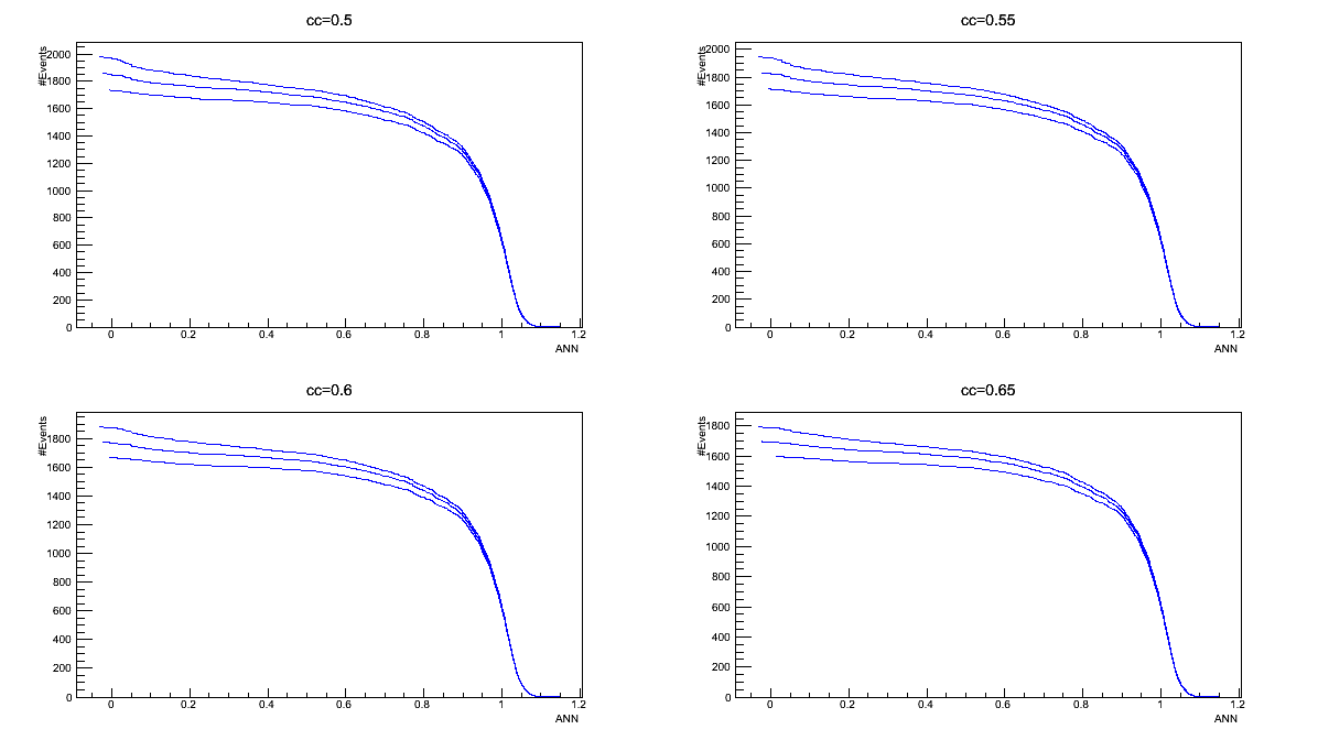
each graph contains ten different curves concerning different thresholds on ANN \ output parameter:
- to the red curve corresponds no cut on ANN \ output
- to the green curves correspond threshold values in the interval [0.2-1] with steps of 0.1;
Only events with \( ANN\output>ANN\ output_{th} \)in the graphs;
The picture names contain the (*) symbol to sign the presence of string which depends on the peculiar characteristcs of the test. In all the cases the
* replaces the name of the root-file which contains the ANN; * replaces the name of the root-file which contains the events for the test; * replaces the ANN output interval used for the creation of the 3. and 4. pictures; * replaces an index (uf) value which is: 0 if the test-file is not the input-file; any other number otherwise.
File for Test an ANN-Use
To use the - Test0_dANN_var.C file and test the ANN you need to know:
ANN-Equipment
In the location where the file and test the ANN you need to know: file is used, the following directories must exist:
- outfile: this directory collects the output files (one for each test) which contain the data;
- ANNthres: this directory collects the pictures 1 and 2 at this section.
- logN_rho: this directory collects the pictures 3 and 4 at this section.
- CC_RHO_ANN_Plots: this directory collects the picture 5 at this section.
ANN-commands
The generic command is:
root -l -b 'Test0_dANN_var_norm.C+("path/..NN/NN_FILE.root","path/..nnTREE/TEST_FILE,
            # SIG-events for test, # BKG-events to test, start-SIG, start-BKG, uf)'
path/..NN/NN_FILE.root: this argument defines the file which contains the ANN which you are going to test. path/..nnTREE/TEST_FILE: this argument defines the test-file which contains the events that you are going to analyse. This file must be built following the previous steps. # SIG/BKG-events for test (TS/BG): this number defines how many examples belonging to the SIG/BKG class you are going to analyse to test the ANN performances. The default value is set to 0; when TS=0 and TB=0 the number of the considered events is the minimum between the total ones of the SIG and the BKG classes. start-SIG/BKG (s/b): this number establishes the first SIG/BKG-event selected to test ANN. All the events in the test-file are tagged by an increasing index, used to identify them. The other TS-1/TB-1 examples are selected from this starting point, following their order in the test-file. The default value is set to 0; when s=0/b=0 the first considered SIG/BKG-event is the first of the list. uf: this number represents an index value which must be: 0 if the test-file is not the input-file; any other number otherwise.
root -l -b 'Test0_dANN_var.C+("NN/8x8Sig_Bkg_mlpNetwork_nTS16384_nTB16384_structure16_32_16_lm5_epochs650_s0_b1200000_ROC.root",
                         "nnTREE/nnTree_NN_CFT01mod_GaussianNoise_SIM_run3_BKG.root",10,10,0,0,0)'
You can find the - Test0_dANN_var.C file and the necessary directories here: /home/waveburst/ANN/Summary/TEST/TestANN.
ANN Average
To improve the SIG and BKG discrimination can be use the - Average.C The main task of this script is to use several ANNs to final judge each event. To achieve this aim the outputs are averaged and the result is use to classify the event. |
| File for averaging ANN outputs-Explanation: |
| File for averaging ANN outputs-Use: |
File for averaging ANN outputs-Explanation
N_ANN_S_*.png (only SIG events)
three different curves concern different thresholds on rho and cc parameter: \( rho_{th}= \) survive the cuts and are taken into account in the graphs;
three different curves concern different thresholds on rho and cc parameter: \( rho_{th}=\) survive the cuts and are taken into account in the graphs;
each graph contains ten different curves concerning different thresholds on ANN average parameter:
- to the red curve corresponds no cut on ANN average;
- to the green curves correspond threshold values in the interval [0.2-1] with steps of 0.1;
Only events with \(ANNaverage>ANNaverage_{th} \)
each graph contains ten different curves concerning different thresholds on ANN average parameter:
- to the red curve corresponds no cut on ANN average;
- to the green curves correspond threshold values in the interval [0.2-1] with steps of 0.1;
Only events with \( ANNaverage>ANNaverage_{th} \)
Mchirp is an estimate of the chirp-mass, obtained through a fitting technique. Obviously this parameter and this comparison is useful only if you are interested in recognizing chirp-like events. The value of this parameter is always calculated for each event by the standard cWB analysis;
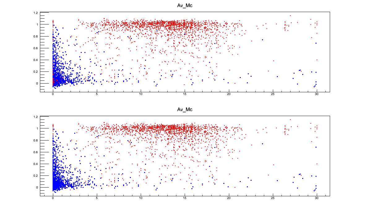
image135|
- ordinates = average on ANN outputs abscissa = cc
The picture names contain the (*) symbol to sign the presence of a string which depends on the decided output name of the test. It is defined as argument of the
ANN Tests
- the
- Test_rho_cc_out1_out2.C file in the directory *Comparison*: it can be used to compare the preformances of two different ANNs;
- Test0_dANN_var_norm.C and
- Test0_dANN_var_norm_neg.C files in the directory *Diff_NORM*: the elements of each frame are differently normalized according to their maximum and minimum values. The first file normalizes the inputs in a range [0,1] the second in the range [-1,1]
- Fisher_1.C file in the directory *Fisher*: this file create an algorithm which finds the Fisher distriminant between the BKG and the SIG events in the ANN output-cc plane. Then it tests this tool on another set of data;
- Test0_Mchirp.C file in the directory *Mchirp*: this file is the analogous of the Test0_dANN_var.C file but the analysis concern the Mchirp parameter instead of the ANN output.