Line & Noise Removal

This page provides a description of the regression.cc class Further documentation is available at the following link:

• Regression-documents: List of presentations and documents

Overview

Regressions enables the subtraction of noise features from a target channel based on the output of one or more auxiliary channels (see the documents above for how it works). The calculation is conducted over narrow sub-bands (layers) of the total bandwidth of the target channel, with a desired frequency resolution. Performing the calculation over sub-bands simplifies the problem, reducing the calculation from a big filter to small ones. Regression also enables the possibility to consider select the appropriate auxiliary channels for in different frequency bands. Finally, the output of several auxiliary channels can be used to perform multi-correlation analysis.

We introduce the following name convention for each single layer:

• h: target (must be a discrete time series)
• s: prediction
• x: one or more auxiliary channels, M is the number of auxiliary channels
• a: filter, with length 2L+1
• R: autocorrelation matrix (2n*2n dimension, n=M(2L+1))
• C: cross-correlation vector (2n=2M(2L+1) dimension)
• Lambda, P: eigen-values and eigen-vectors matrices related to R (2n*2n dimension, n=M(2L+1))
• Lambda’: eigen-values matrix after the application of the regolators

Implementation

The regression class is implemented in the WAT library and contains the following C++ struct :

• Wiener: a structure which contains the values of the filter a.

The following list reports the attributes of regression object:

• kSIZE: the value of L (half-length of filter)
• Edge: a scratch time applied to the boundaries of segment
• chList: WSeries for each channel
• chName: names of the channels
• chMask: integers storing the frequency layers for each channel shouldbe used
• FILTER: Wiener struct storing the filter for each layer
• matrix: matrix R for each layer
• vCROSS: cross-correlation vector C for each layer
• vEIGEN: matrix Lambda’ for each layer
• target: target time series
• rnoise: prediction (s) in time domain
• WNoise: prediction (s) in Time-Frequency domain
• vrank: rank contribution for each layer and for each channel
• vfreq: central frequency of each layer

A number of functions has been written for the regression method. These are classified into the following groups:

Object Definition	Constructor and destructor
Channels definition	Inserting target and auxiliary channel
Filter calculation	Calculation of R,C,a,s
Getting attributes	Getting attributes
Linear Predictor Estimator	Using regression as LPE

Examples

This section reports an example of an analysis performed with the regression method.

Regression Examples	Regression examples
NMAPI integration	Integration in NMAPI Virgo tool

Regression examples

Test on Gaussian noise

In these examples target and witness channels are combination of gaussian noises.
These tests have been suggested by reviewers.
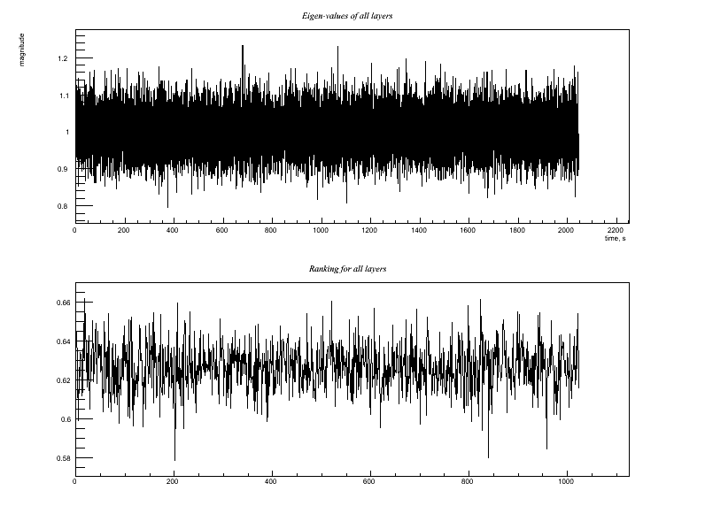
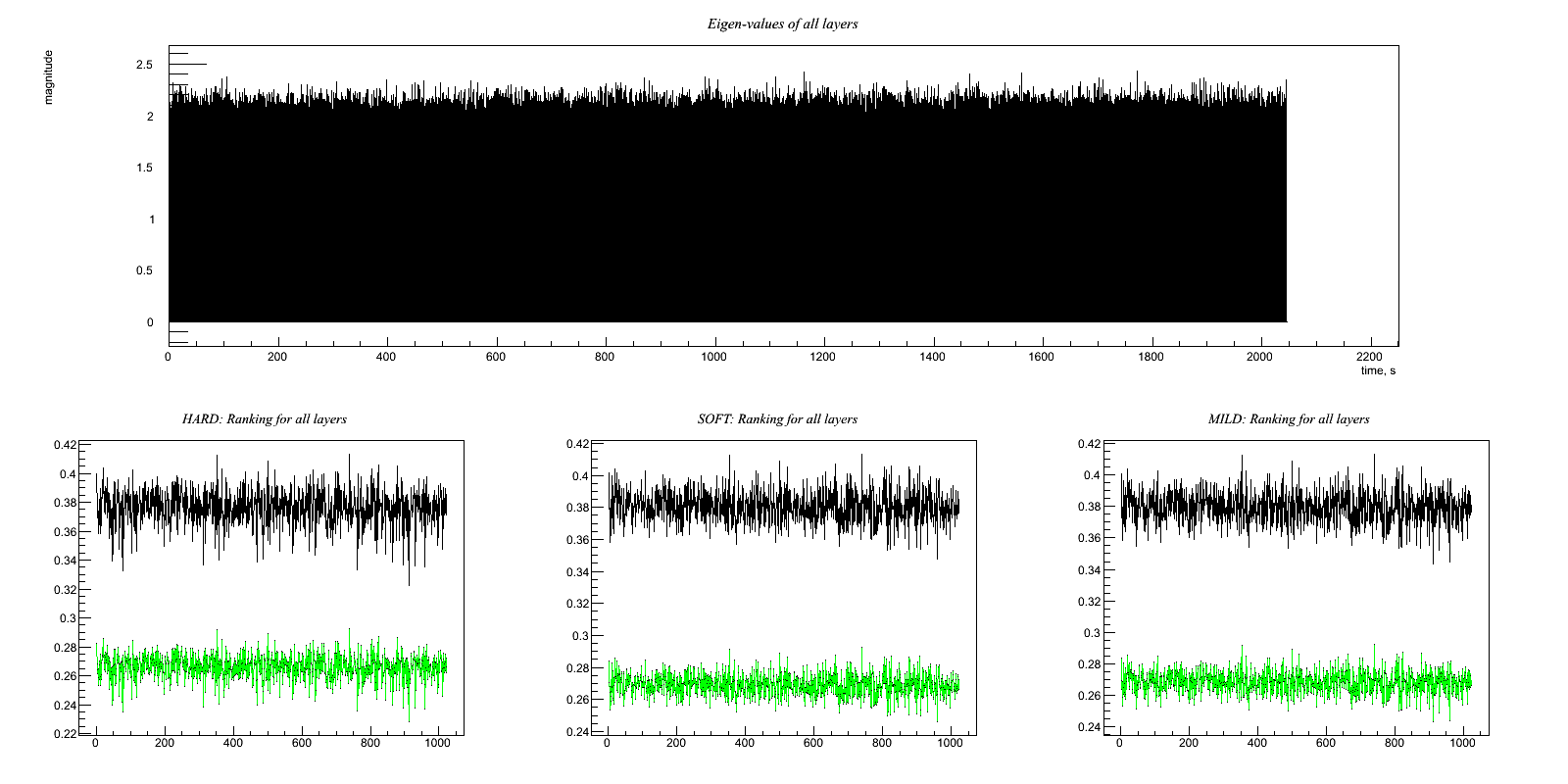
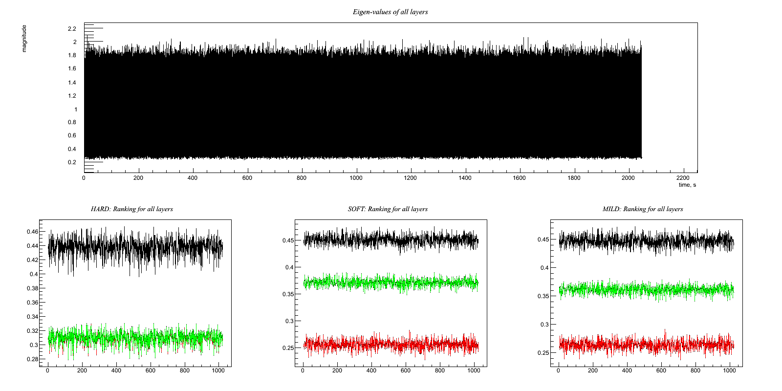
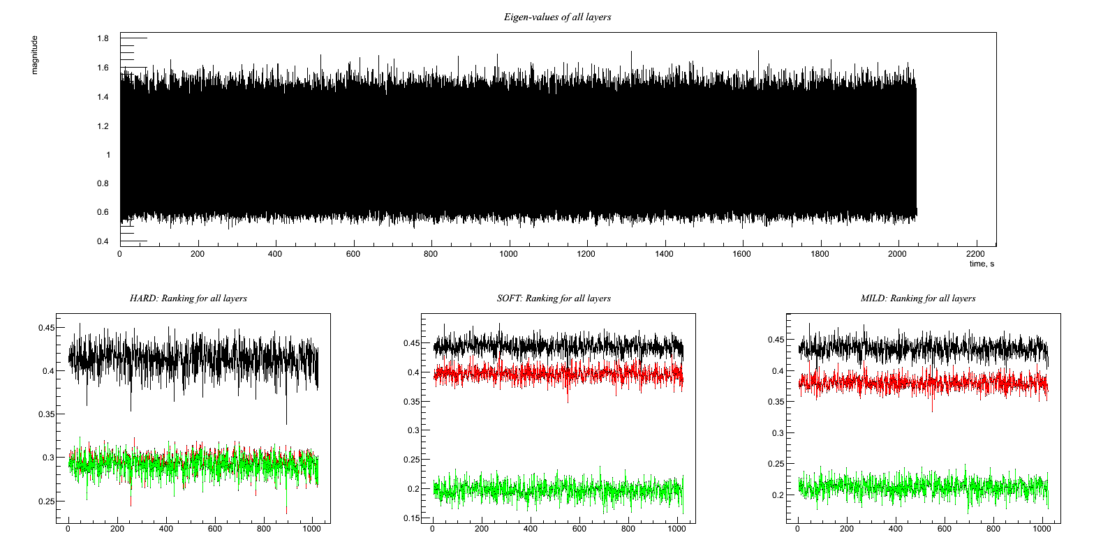
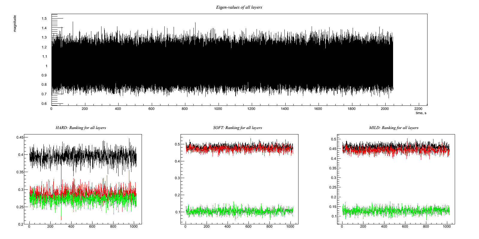
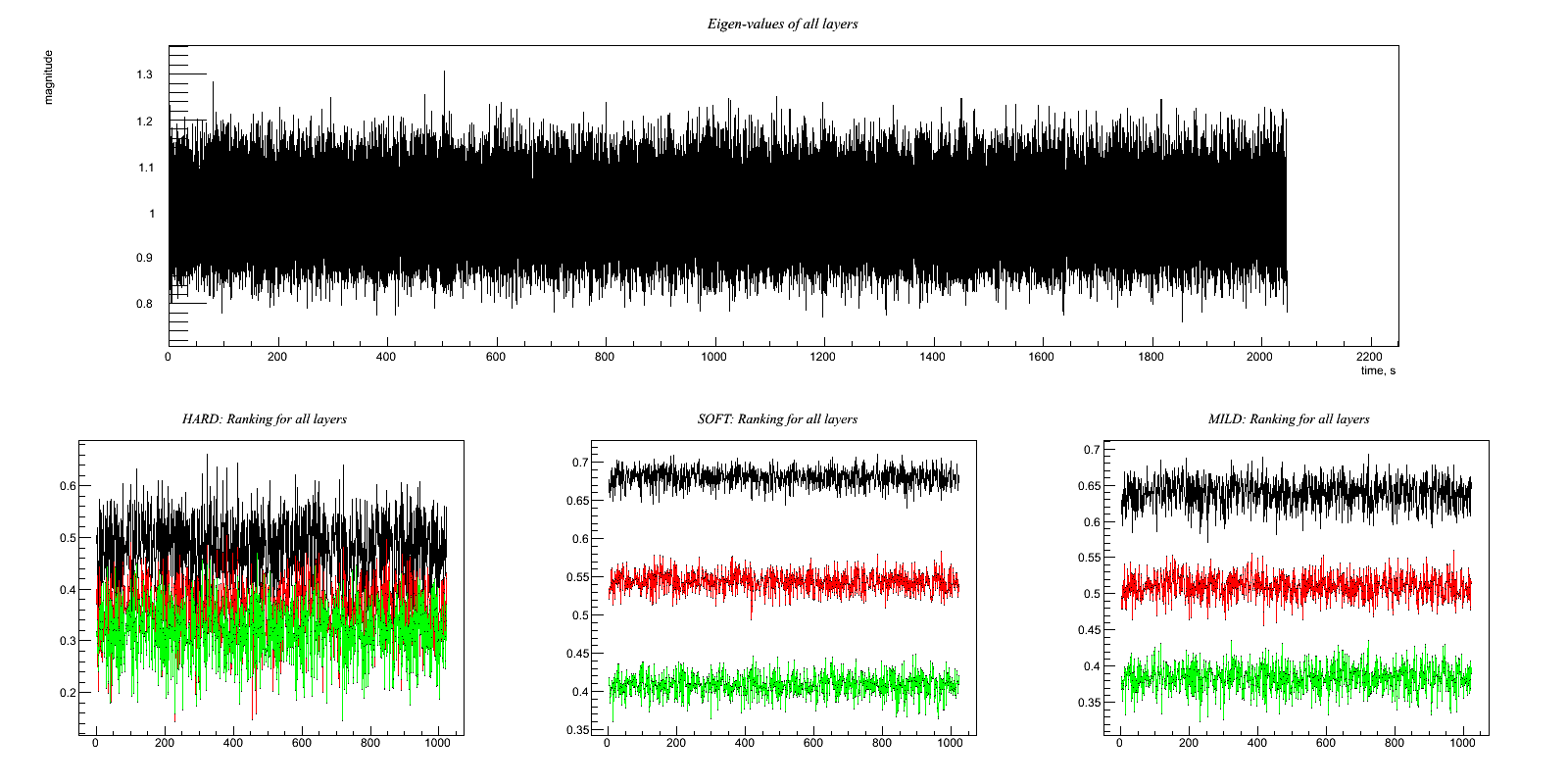
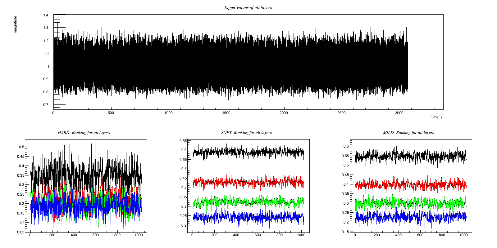
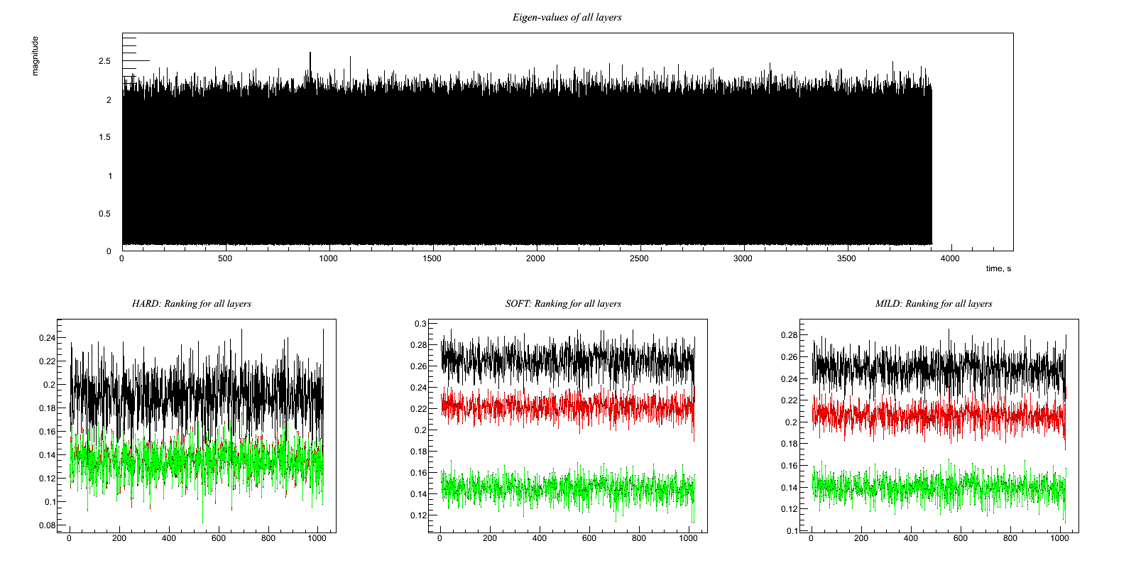
We report for each test a plot containing eigen-values and rank for each witness channel.

Usually target channel is sort of type: H = x + w
where w is noise to be cleaned.
So each script report at the end mean and rms of the following time series:
- x
- clean
- clean-x
This because x and clean should be the same channel, instead clean-x should be 0.

• Test1.C Removal of broadband noise using a single, highly correlated witness channel. Output:

  Removal of broadband noise using a single, highly correlated witness channel.
  You can prepare the channels with the desired correlation this way, for instance:
  Generate time series w(t) and x(t) each containing Gaussian white noise (unit variance)
  Construct the witness channel: A(t) = w(t)
  Construct the target channel:  H(t) = x(t) + 0.8*w(t)
  Compare the ASD (or simply the RMS) of H(t) before and after regression.
  The regression should be able to reduce the noise amplitude by a factor of
       1/sqrt(1^2+0.8^2) = 1/sqrt(1.64) ~ 0.78
  

  Results:

  Ratio rms: (0.998905/1.28003)= 0.780374
  x         : 0.000118281 0.999683
  clean     : -0.000804828 0.998905
  clean-x   : -0.000923109 0.0817862
  

  
  

  

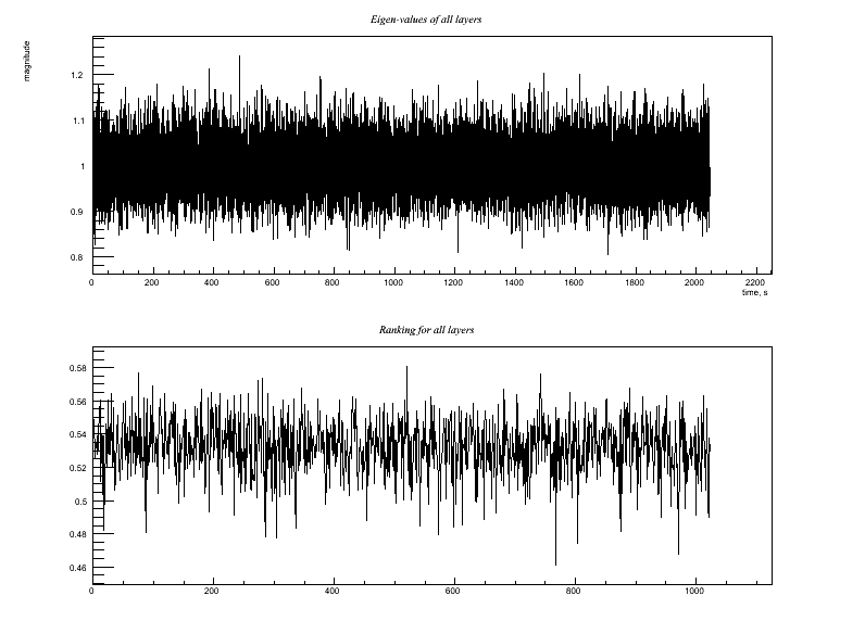
• Test2.C Similar, but witness channel includes some uncorrelated noise: Output:

  Test 2: Similar, but witness channel includes some uncorrelated noise:
  Generate white noise time series w(t), x(t), y(t)
  Witness channel: A(t) = 0.6*y(t) + w(t)
  Target channel:  H(t) = x(t) + 0.8*w(t)
  Compare the ASD (or simply the RMS) of H(t) before and after regression.
  Since regression removes the w(t) correlated noise but adds in some y(t)
  noise from the witness channel, I think the regression should be able to
  reduce the noise amplitude by a factor of
       sqrt(1^2+(0.8*0.6)^2)/sqrt(1^2+0.8^2) = sqrt(1.23)/sqrt(1.64) ~ 0.87
  

  Results:

  Ratio rms: (1.08211/1.2814)= 0.844474
  x         : 1.49279e-05 1.00022
  clean     : 0.000703435 1.08211
  clean-x   : 0.000688507 0.423346
  

  
  

  

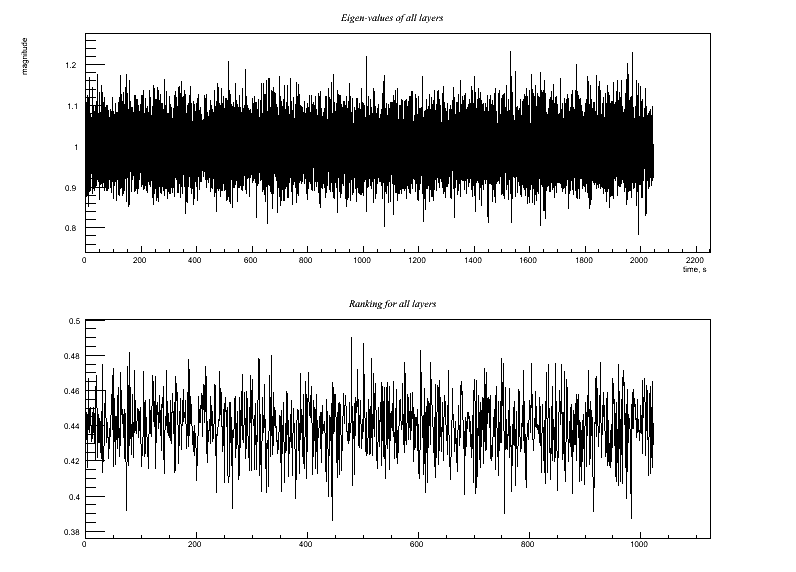
• Test3.C Similar, but witness channel includes more uncorrelated noise: Output:

  Test 3: Similar, but witness channel includes more uncorrelated noise:
  Witness channel: A(t) = y(t) + w(t)
  Target channel:  H(t) = x(t) + 0.8*w(t)
  Compare the ASD (or simply the RMS) of H(t) before and after regression.
  Since regression removes the w(t) correlated noise but adds an equal
  amount of y(t) noise, it should not be able to reduce the noise amplitude in H(t).
  

  Results:

  Ratio rms: (1.14762/1.27984)= 0.896693
  x         : -0.000137184 0.999029
  clean     : 0.000252871 1.14762
  clean-x   : 0.000390055 0.572221
  

  
  

  

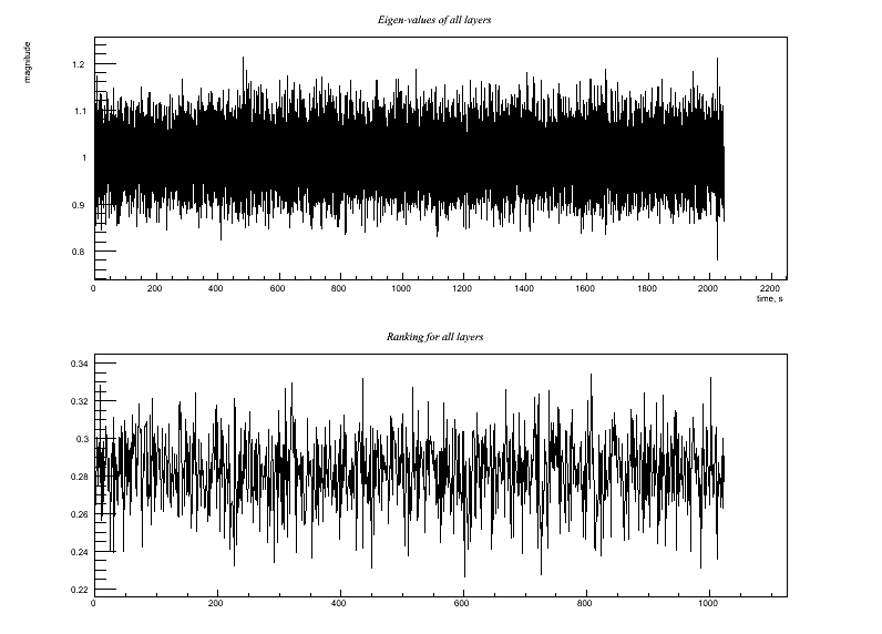
• Test4.C Similar, but witness channel has mostly uncorrelated noise. Output:

  Test 4: Similar, but witness channel has mostly uncorrelated noise.
  Witness channel: A(t) = y(t) + 0.5*w(t)
  Target channel:  H(t) = x(t) + 0.8*w(t)
  Trying to do regression would add more noise that it removes.  Is the code smart
  enough to determine this and choose NOT to use this witness channel for regression?
  

  Results:

  Ratio rms: (1.22895/1.28215)= 0.958502
  x         : 0.000117791 1.00031
  clean     : 0.000277306 1.22895
  clean-x   : 0.000159515 0.718146
  

  
  

  

• Test5.C Two identical (i.e., redundant) witness channels: Output:

  Test 5: Two identical (i.e., redundant) witness channels:
  Witness channels: A(t) = 0.6*y(t) + w(t)
                    B(t) = A(t)
  Target channel:   H(t) = x(t) + 0.8*w(t)
  This could be pathological in terms of matrix inversion, but corresponds to a very
  realistic case of, say, two power-line monitors (with high signal-to-noise) both
  showing 60 Hz and harmonics, equivalently.  The right answer in terms of the
  regression goal is that we can use EITHER A(t) or B(t) (or any linear combination
  of them) and achieve the same result as Test 2 above.  In other words, I'd like to
  think that it is harmless to include extra redundant aux channels.  So does the
  code manage to do that?
  * Try this with hard, soft, and mild regulators *
  

  Results:

  HARD:
  Ratio rms: (1.08188/1.28075)= 0.844727
  x         : -0.00086732 0.99952
  clean     : -0.000774834 1.08188
  clean-x   : 9.24859e-05 0.423357
  -------------------
  SOFT:
  Ratio rms: (1.07976/1.28075)= 0.843067
  x         : -0.00086732 0.99952
  clean     : -0.0007748 1.07976
  clean-x   : 9.25191e-05 0.418084
  -------------------
  MILD:
  Ratio rms: (1.07982/1.28075)= 0.843122
  x         : -0.00086732 0.99952
  clean     : -0.000774804 1.07982
  clean-x   : 9.2516e-05 0.418233
  -------------------
  

  
  

  

• Test6.C Two witness channels, one highly correlated and the other not Output:

  Test 6: Two witness channels, one highly correlated and the other not
  Witness channels: A(t) = y(t) + w(t)
                    B(t) = w(t)
  Target channel:   H(t) = x(t) + 0.8*w(t)
  Hopefully, the code figures out that it should use B(t) in the regression and
  ignore A(t).  The net reduction in noise should be the same as Test 1 above.
  * Try this with hard, soft, and mild regulators *
  

  Results:

  HARD:
  Ratio rms: (1.04764/1.28094)= 0.81787
  x         : -0.000725006 1.00052
  clean     : -0.000114259 1.04764
  clean-x   : 0.000610748 0.323453
  -------------------
  SOFT:
  Ratio rms: (1.02945/1.28094)= 0.803672
  x         : -0.000725006 1.00052
  clean     : -0.000114251 1.02945
  clean-x   : 0.000610755 0.262148
  -------------------
  MILD:
  Ratio rms: (1.03179/1.28094)= 0.805497
  x         : -0.000725006 1.00052
  clean     : -0.000114252 1.03179
  clean-x   : 0.000610755 0.270657
  -------------------
  

  
  

  

• Test7.C One witness channel with a little uncorrelated noise, other with more Output:

  Test 7: One witness channel with a little uncorrelated noise, other with more
  Generate white noise time series w(t), x(t), y(t), z(t)
  Witness channels: A(t) = 0.6*y(t) + w(t)
                    B(t) = z(t) + 0.5*w(t)
  Target channel:   H(t) = x(t) + 0.8*w(t)
  Hopefully, the code figures out that it should use A(t) and ignore B(t).  The net
  reduction in noise should be the same as Test 2 above.
  * Try this with hard, soft, and mild regulators *
  

  Results:

  HARD:
  Ratio rms: (1.11732/1.28115)= 0.872121
  x         : 0.000533018 1.00039
  clean     : 0.000452029 1.11732
  clean-x   : -8.09883e-05 0.504925
  -------------------
  SOFT:
  Ratio rms: (1.08964/1.28115)= 0.85052
  x         : 0.000533018 1.00039
  clean     : 0.000451997 1.08964
  clean-x   : -8.10209e-05 0.445032
  -------------------
  MILD:
  Ratio rms: (1.08957/1.28115)= 0.850462
  x         : 0.000533018 1.00039
  clean     : 0.000452054 1.08957
  clean-x   : -8.0964e-05 0.445399
  -------------------
  

  
  

  

• Test8.C Similar, but second witness channel has a very small (but nonzero) correlation Output:

  Test 8: Similar, but second witness channel has a very small (but nonzero) correlation
  Witness channels: A(t) = 0.6*y(t) + w(t)
                    B(t) = z(t) + 0.2*w(t)
  Target channel:   H(t) = x(t) + 0.8*w(t)
  Hopefully, the code will give the same result as tests 2 and 7 -- i.e. ignore B(t),
  since trying to use it in the regression would only add noise.
  * Try this with hard, soft, and mild regulators *
  

  Results:

  HARD:
  Ratio rms: (1.15622/1.2816)= 0.902168
  x         : 9.92543e-05 1.00016
  clean     : 0.00050095 1.15622
  clean-x   : 0.000401696 0.586336
  -------------------
  SOFT:
  Ratio rms: (1.08418/1.2816)= 0.84596
  x         : 9.92543e-05 1.00016
  clean     : 0.000501103 1.08418
  clean-x   : 0.000401849 0.426438
  -------------------
  MILD:
  Ratio rms: (1.08815/1.2816)= 0.849059
  x         : 9.92543e-05 1.00016
  clean     : 0.000501097 1.08815
  clean-x   : 0.000401843 0.435835
  -------------------
  

  
  

  

• Test9.C Two good witness channels measuring different effects Output:

  Test 9: Two good witness channels measuring different effects
  Witness channels: A(t) = w(t)
                    B(t) = v(t)
  Target channel:   H(t) = x(t) + 0.8*w(t) + 0.6*v(t)
  Compare the ASD (or simply the RMS) of H(t) before and after regression.
  The regression should be able to reduce the noise amplitude by a factor of
       1/sqrt(1^2+0.8^2+0.6^2) = 1/sqrt(2.00) ~ 0.71
  

  Results:

  HARD:
  Ratio rms: (1.21678/1.41389)= 0.860593
  x         : 0.000298055 0.999962
  clean     : -0.000296588 1.21678
  clean-x   : -0.000594643 0.69913
  -------------------
  SOFT:
  Ratio rms: (1.00004/1.41389)= 0.707296
  x         : 0.000298055 0.999962
  clean     : -0.000296922 1.00004
  clean-x   : -0.000594977 0.126131
  -------------------
  MILD:
  Ratio rms: (1.00791/1.41389)= 0.712862
  x         : 0.000298055 0.999962
  clean     : -0.000296866 1.00791
  clean-x   : -0.000594921 0.175355
  -------------------
  

  
  

  

• Test10.C Two good witness channels plus one slightly correlated one Output:

  Test 10: Two good witness channels plus one slightly correlated one
  Witness channels: A(t) = w(t)
                    B(t) = v(t)
                    C(t) = y(t) + 0.5*z(t)
  Target channel:   H(t) = x(t) + 0.8*w(t) + 0.6*v(t) + z(t)
  Compare the ASD (or simply the RMS) of H(t) before and after regression.
  Although C(t) is correlated, using it in the regression would add more noise than
  it removes.  So hopefully the code will use A and B to regress but ignore C.
  The result, then, should be the same as Test 9.
  * Try this with hard, soft, and mild regulators *
  

  Results:

  HARD:
  Ratio rms: (1.64183/1.73322)= 0.947273
  x         : -0.00166639 0.999727
  clean     : -0.00175032 1.64183
  clean-x   : -8.39278e-05 1.3037
  -------------------
  SOFT:
  Ratio rms: (1.34039/1.73322)= 0.773353
  x         : -0.00166639 0.999727
  clean     : -0.00175059 1.34039
  clean-x   : -8.42073e-05 0.905124
  -------------------
  MILD:
  Ratio rms: (1.35391/1.73322)= 0.781153
  x         : -0.00166639 0.999727
  clean     : -0.00175052 1.35391
  clean-x   : -8.41311e-05 0.924155
  -------------------
  

  
  

  

• Test11.C Two witness channels have some common noise (or environmental signal, but anyway uncorrelated with the GW target channel) between them Output:

  Test 11: Two witness channels have some common noise (or environmental signal,
  but anyway uncorrelated with the GW target channel) between them
  Witness channels: A(t) = 0.4*y(t) + w(t) + v(t)
                    B(t) = 0.2*z(t) + 0.5*w(t) + v(t)
  Target channel:   H(t) = x(t) + 0.8*w(t)
  Hopefully, the code figures out that it should subtract a linear combination of
  A(t) and B(t).  If I've done the math right (on paper), the optimal combination is
  (0.9933)A(t)-(0.7726)B(t).  Note that the v(t) noise mostly (but not completely)
  cancels out in that combination.  The w(t) component amplitude in H(t) reduces
  from 0.8 to 0.195, although the post-regression H(t) also picks up amplitudes
  of 0.4*0.9933=0.3973 from the y(t) term in A(t), 0.2*0.7726=0.1545 from the z(t)
  term in B(t), and 0.9933-0.7726=0.2207 from the combined v(t) terms.  So the
  expected reduction in noise amplitude is by a factor of
        sqrt(1+(0.195)^2+(0.3973)^2+(0.1545)^2+(0.2207)^2)/sqrt(1^2+0.8^2)
        = sqrt(1.268)/sqrt(1.64) = 0.88
  * Try this with hard, soft, and mild regulators *
  

  Results:

  HARD:
  Ratio rms: (1.27988/1.28007)= 0.999849
  x         : -2.18285e-05 0.999655
  clean     : 0.00017788 1.27988
  clean-x   : 0.000199708 0.799899
  -------------------
  SOFT:
  Ratio rms: (1.1867/1.28007)= 0.927054
  x         : -2.18285e-05 0.999655
  clean     : 0.000177879 1.1867
  clean-x   : 0.000199707 0.646697
  -------------------
  MILD:
  Ratio rms: (1.21162/1.28007)= 0.946523
  x         : -2.18285e-05 0.999655
  clean     : 0.000177878 1.21162
  clean-x   : 0.000199707 0.69103
  -------------------
  

  
  

  

Test on Sinusoidal signal injected in Gaussian noise

In these examples target and witness channels are gaussian noise containing a sinusoidal signal

• Regression_Sine.C Clean a sine at 100 Hz . Output:

  
  

  

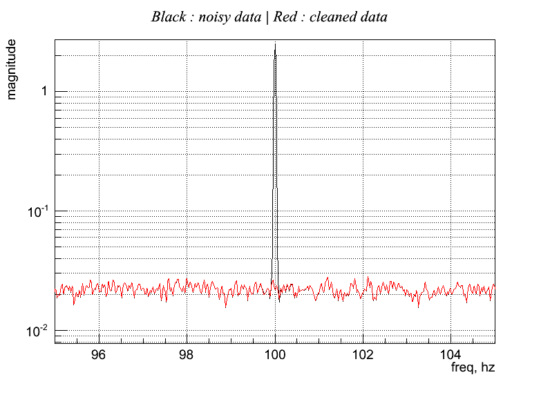
  This example write also the rank values and eigenvalues for each layer. Note that in the layers containing only noise the eigen-values are near to one, while in the layer of the sine the eigen-values are very different, and only the biggest are important.

  Ranking (freq - rank):
  96 0.0380424
  97 0.0276262
  98 0.0240649
  99 0.0140932
  100 0.706418
  101 0.0324515
  102 0.0206146
  103 0.00714935
  104 0.0321715
  
  Eigen-values at frequency layer (first line is frequency, than eigen-values)
     96      97      98      99     100     101     102     103     104
  
  1.110   1.077   1.113   1.073   5.999   1.155   1.071   1.103   1.077
  1.110   1.077   1.113   1.073   5.999   1.155   1.071   1.103   1.077
  1.092   1.037   1.092   1.065   4.999   1.134   1.059   1.088   1.065
  1.092   1.037   1.092   1.065   4.999   1.134   1.059   1.088   1.065
  1.045   1.027   1.036   1.055   0.000   1.076   1.040   1.053   1.057
  1.045   1.027   1.036   1.055   0.000   1.076   1.040   1.053   1.057
  1.026   1.016   1.022   1.029   0.000   1.036   1.035   1.031   1.034
  1.026   1.016   1.022   1.029   0.000   1.036   1.035   1.031   1.034
  1.013   1.010   1.015   1.001   0.000   0.987   1.034   1.027   1.003
  1.013   1.010   1.015   1.001   0.000   0.987   1.034   1.027   1.003
  1.002   0.998   0.999   1.000   0.000   0.976   1.009   1.007   0.976
  1.002   0.998   0.999   1.000   0.000   0.976   1.009   1.007   0.976
  0.976   0.986   0.969   0.993   0.000   0.947   0.988   0.993   0.970
  0.976   0.986   0.969   0.993   0.000   0.947   0.988   0.993   0.970
  0.953   0.975   0.968   0.972   0.000   0.934   0.964   0.982   0.969
  0.953   0.975   0.968   0.972   0.000   0.934   0.964   0.982   0.969
  0.948   0.963   0.955   0.952   0.000   0.928   0.951   0.957   0.966
  0.948   0.963   0.955   0.952   0.000   0.928   0.951   0.957   0.966
  0.932   0.957   0.920   0.934   0.000   0.919   0.933   0.886   0.954
  0.932   0.957   0.920   0.934   0.000   0.919   0.933   0.886   0.954
  0.904   0.953   0.911   0.926   0.000   0.908   0.916   0.873   0.931
  0.904   0.953   0.911   0.926   0.000   0.908   0.916   0.873   0.931
  

• Regression_Sine_parameters.C Clean a sine at 100 Hz . Output: See the difference on parameters:

  
  

  

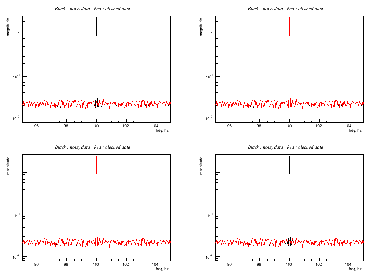
  This example shown some changes on the regression parameters showing some conditions which avoid the line cleaning.

  • Top left:

    r.setFilter(5);
    r.setMatrix(totalscratch);
    r.solve(0., 4, 'h');
    r.apply(0.2);
    

  • Top right: same as top left except for:

    r2.apply(0.8);
    

    Rank for layer = 100 Hz is 0.7, putting a threshold of 0.8 discard the use of this layer: line is not cleaned

  • Bottom left: same as top left except for:

    r3.solve(0, 2, 'h');
    

    This select only the first 2 eigen-values, which are not enough to describe the line: not cleaned

  • Bottom right: same as top left except for:

    r4.setFilter(2);
    

    The filter is too short to describe the prediction: line is not cleaned

• Regression_Sine_Bic.C Clean a sine at 100 +/- 2 Hz using multi-linear correlation. Output:

  
  

  

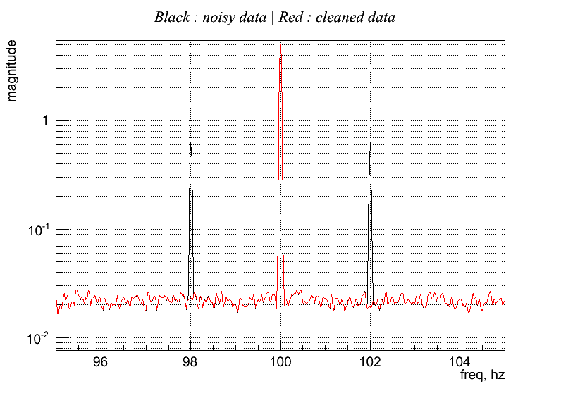
  Note that in this example we DID not clean the carrier line at 100 Hz. Same consideration about rank and eigen-values of previous example are now applied at the frequencies 100 +/- 2Hz

  Ranking (freq - rank):
  96 0.0182773
  97 0.028398
  98 0.69655
  99 0.0195045
  100 0.018786
  101 0.013739
  102 0.696316
  103 0.0152138
  104 0.00614439
  
  Eigen-values at frequency layer (first line is frequency, than eigen-values)
     96      97      98      99     100     101     102     103     104
  
  1.051   1.050   5.988   1.112   1.099   1.133   5.988   1.082   1.057
  1.051   1.050   5.988   1.112   1.099   1.133   5.988   1.082   1.057
  1.038   1.031   4.990   1.095   1.084   1.096   4.990   1.056   1.041
  1.038   1.031   4.990   1.095   1.084   1.096   4.990   1.056   1.041
  1.027   1.015   0.003   1.050   1.059   1.065   0.003   1.044   1.030
  1.027   1.015   0.003   1.050   1.059   1.065   0.003   1.044   1.030
  1.015   1.005   0.003   1.019   1.031   1.053   0.003   1.034   1.030
  1.015   1.005   0.003   1.019   1.031   1.053   0.003   1.034   1.030
  1.007   1.004   0.003   0.992   1.010   1.016   0.003   1.017   1.029
  1.007   1.004   0.003   0.992   1.010   1.016   0.003   1.017   1.029
  1.003   1.003   0.003   0.983   0.984   0.994   0.003   0.995   1.016
  1.003   1.003   0.003   0.983   0.984   0.994   0.003   0.995   1.016
  1.001   0.985   0.002   0.981   0.969   0.982   0.003   0.985   1.001
  1.001   0.985   0.002   0.981   0.969   0.982   0.003   0.985   1.001
  0.995   0.981   0.002   0.950   0.967   0.941   0.002   0.980   0.997
  0.995   0.981   0.002   0.950   0.967   0.941   0.002   0.980   0.997
  0.966   0.977   0.002   0.947   0.953   0.921   0.002   0.966   0.981
  0.966   0.977   0.002   0.947   0.953   0.921   0.002   0.966   0.981
  0.956   0.975   0.002   0.942   0.930   0.903   0.002   0.927   0.918
  0.956   0.975   0.002   0.942   0.930   0.903   0.002   0.927   0.918
  0.940   0.971   0.002   0.929   0.915   0.895   0.002   0.913   0.900
  0.940   0.971   0.002   0.929   0.915   0.895   0.002   0.913   0.900
  

• Regression_Sine_Gaus_Bic.C Clean a Gaussian noise up-converted with a 100 Hz line carrier. Output:

  
  

  

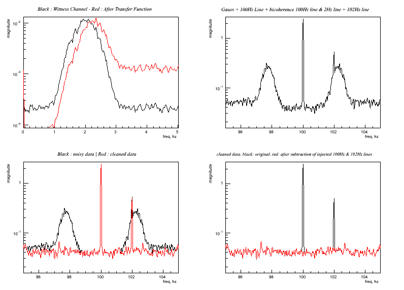
  Ranking (freq - rank):
  95.5 0.637558
  96 0.643526
  96.5 0.642644
  97 0.822235
  97.5 0.973241
  98 0.967509
  98.5 0.790975
  99 0.170191
  99.5 0.0908794
  100 0.00781286
  100.5 0.0615298
  101 0.140019
  101.5 0.769942
  102 0.788914
  102.5 0.971866
  103 0.813191
  103.5 0.634377
  104 0.65289
  104.5 0.641887
  
  Eigen-values at frequency layer (first line is frequency, than eigen-values)
   95.5      96    96.5      97    97.5      98    98.5      99    99.5     100   100.5     101   101.5     102   102.5    103   103.5     104   104.5
  
  1.147   1.115   1.194   2.478   2.206   1.167   2.199   2.801   1.120   1.351   1.121   2.795   2.198   1.159   2.184 2.506    1.182   1.111   1.151
  1.147   1.115   1.194   2.478   2.206   1.167   2.199   2.801   1.120   1.351   1.121   2.795   2.198   1.159   2.184 2.506    1.182   1.111   1.151
  1.124   1.075   1.167   2.355   2.135   1.150   2.092   2.585   1.103   1.081   1.104   2.578   2.089   1.145   2.116 2.382    1.156   1.080   1.134
  1.124   1.075   1.167   2.355   2.135   1.150   2.092   2.585   1.103   1.081   1.104   2.578   2.089   1.145   2.116 2.382    1.156   1.080   1.134
  1.095   1.072   1.069   1.604   1.617   1.127   1.460   1.435   1.068   1.075   1.065   1.422   1.451   1.134   1.624 1.603    1.063   1.071   1.106
  1.095   1.072   1.069   1.604   1.617   1.127   1.460   1.435   1.068   1.075   1.065   1.422   1.451   1.134   1.624 1.603    1.063   1.071   1.106
  1.041   1.069   1.026   1.374   1.376   1.123   1.298   1.197   1.057   0.995   1.059   1.191   1.295   1.132   1.386 1.365    1.025   1.071   1.048
  1.041   1.069   1.026   1.374   1.376   1.123   1.298   1.197   1.057   0.995   1.059   1.191   1.295   1.132   1.386 1.365    1.025   1.071   1.048
  0.999   1.055   1.006   0.911   1.004   1.086   0.980   0.779   1.044   0.992   1.045   0.789   0.991   1.093   1.017 0.900    1.006   1.055   1.000
  0.999   1.055   1.006   0.911   1.004   1.086   0.980   0.779   1.044   0.992   1.045   0.789   0.991   1.093   1.017 0.900    1.006   1.055   1.000
  0.984   0.994   0.980   0.652   0.837   1.020   0.838   0.611   1.026   0.976   1.025   0.617   0.843   1.020   0.842 0.645    0.979   0.991   0.990
  0.984   0.994   0.980   0.652   0.837   1.020   0.838   0.611   1.026   0.976   1.025   0.617   0.843   1.020   0.842 0.645    0.979   0.991   0.990
  0.982   0.981   0.958   0.446   0.615   0.968   0.724   0.456   0.984   0.963   0.982   0.457   0.722   0.964   0.614 0.436    0.964   0.981   0.988
  0.982   0.981   0.958   0.446   0.615   0.968   0.724   0.456   0.984   0.963   0.982   0.457   0.722   0.964   0.614 0.436    0.964   0.981   0.988
  0.937   0.954   0.951   0.370   0.424   0.925   0.521   0.343   0.950   0.925   0.945   0.347   0.523   0.920   0.425 0.360    0.962   0.959   0.927
  0.937   0.954   0.951   0.370   0.424   0.925   0.521   0.343   0.950   0.925   0.945   0.347   0.523   0.920   0.425 0.360    0.962   0.959   0.927
  0.918   0.911   0.933   0.327   0.358   0.884   0.419   0.297   0.934   0.911   0.929   0.302   0.421   0.880   0.360 0.321    0.944   0.910   0.906
  0.918   0.911   0.933   0.327   0.358   0.884   0.419   0.297   0.934   0.911   0.929   0.302   0.421   0.880   0.360 0.321    0.944   0.910   0.906
  0.905   0.898   0.872   0.248   0.227   0.791   0.252   0.253   0.866   0.896   0.872   0.256   0.251   0.790   0.230 0.248    0.874   0.897   0.892
  0.905   0.898   0.872   0.248   0.227   0.791   0.252   0.253   0.866   0.896   0.872   0.256   0.251   0.790   0.230 0.248    0.874   0.897   0.892
  0.868   0.875   0.845   0.235   0.199   0.760   0.218   0.243   0.847   0.834   0.854   0.247   0.216   0.763   0.202 0.235    0.845   0.874   0.858
  0.868   0.875   0.845   0.235   0.199   0.760   0.218   0.243   0.847   0.834   0.854   0.247   0.216   0.763   0.202 0.235    0.845   0.874   0.858
  

Real Data

These two scripts need the list of frame files for target and auxiliary channel.
They work on CIT at: /home/drago/Regression-Phase/Review.

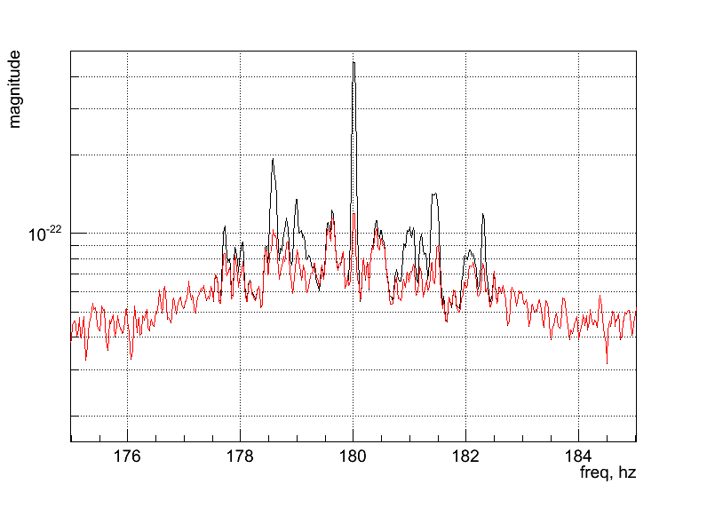
• Regression_H1.C How to apply regression to subtract power line at 180Hz. Output: ( )
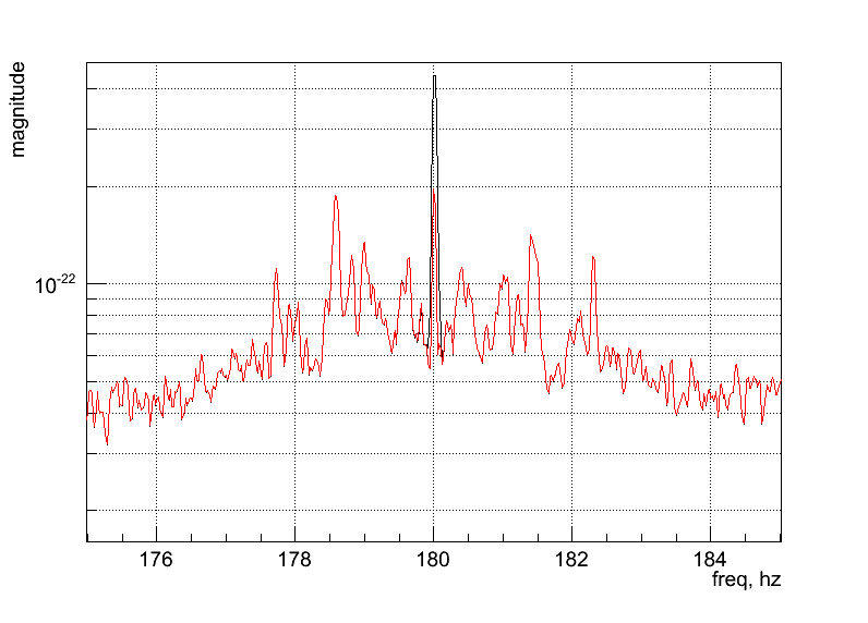
• Regression_H1_bic.C How to apply regression to subtract power line at 180Hz and related sidebands. Output: ( )
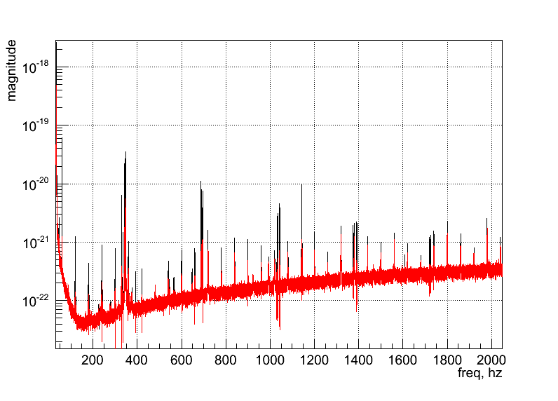
• Regression_H1.C How to apply LPE on all frequency band using regression. Output: ( )

NMAPI integration

Integration in NMAPI Virgo tool

NMAPI (Noise Monitor Application Programming Interface) is a Virgo tool which interfaces various Noise Monitors developed by Virgo scientists. Some documents about NMAPI are in the following links (some are Virgo protected):

• Noise Monitor Application Programming Interface (NMAPI) Software Requirements
• Noise Monitor Applicationrogramming Interface (NMAPI) Development Report
• NMAPI and NoEMi for Advanced Detectors
• Noise Monitor Application rogramming Interface (NMAPI) - Latest developments

All the scripts are located in the Cascina cluster. NMAPI uses condor interface to submit the jobs related for each query received from the web.

Regression integration in NMAPI is dedicated for bilinear correlations of Virgo auxiliary channels with the gravitational one. We considered two carrier channels:

• Pr_power50 for power lines
• V1:Pr_B5_ACp for calibration lines

The results are given in appropriate figure of merits reporting for each frequency band (1Hz resolution, centered at an integer number of frequency) the rank value of the correlation (rank near to 1, high correlation).

Regression in NMAPI involves two different output:

1. Database query: on a set of selected channels.
2. On-the-fly query: on the all possible set of channels.

Database query

The idea is to have an online analysis of bi-linear correlation of a small set of defined channel (about 10-20). After saving the rank values on-the-fly, the user can recall the results for the desired period and channels. The code is split in two parts:

1. The directory which creates the database. An example is on the dir: /users/drago/Regression/VSR4 It is stricly hard-coded, in the example it consider 24 channels on the frequency band of 0-2048 Hz.

2. The script which query the database: /a/st7/storage/d001/web/nmapi/NMAPI_scripts/Regression

   The input parameters are:
   • An identificative number given by NMAPI
   • Auxiliary channel
   • Time period: Start and Stop
   • Frequency band: Low and High
   • Frequency resolution for the output figure (It collects more frequency bins in the same one reporting the maximum value)

   The script file is Regression.sh which calls DrawRankChannel.C

On the fly query

This allows to obtain the bi-linear ranking for each channel in the frame, at a limited period of a single job. The scripts called by NMAPI are located in the directory: /a/st7/storage/d001/web/nmapi/NMAPI_scripts/Regression_QueryChannel. The main script is Regression_QueryChannel.csh which call the macro Regression_QueryChannel.C

• An identificative number given by NMAPI
• Auxiliary channel
• Time period: Start and length
• Frequency band: Low and High
• Ranking threshold of results (write frequencies with rank greater than threshold)

List of constructor and destructor

This page shows the list of functions used by the regression class as object constructors and destructors in the c++ language.

• regression::regression()

  Default constructor

• regression::regression(const regression&)

  Copy constructor from another regression object

• regression::operator_

  Copy constructor from another regression object

• regression::regression(WSeries<double> &, char*, double fL=0., double fH=0.)

  Constructor inserting target channel as a WSeries object. It calls the

• regression::add() function. See also Channels definition

• regression::clear()

  Clear the regression object. All the inserted channels are removed.

• regression::_regression

  Default distructor. It calls the function clear()

Inserting target and auxiliary channels

Target channel is the base channel for all the procedure. This is defined in the regression specifying a TF resolution, which is used for all the auxiliary channels. This is done using a WSeries class, which contains the TF transform of target data.

Target channel defines also the maximum frequency band in which the regression is applied. Auxiliary channels are inserted using wavearray objects. It is possible to define limited frequency bands for each auxiliary channel, so to specialize each auxiliary channel and limit the computational coast.

• regression::add(WSeries<double> & target, char* name, double fL=0., double fH=0.) Add the target channel. It is possible to specify a desired frequency band. If not, all the frequency band of the target is considered.

• regression::add(wavearray<double>& witness, char* name, double fL=0., double fH=0.) Add one auxiliary channel. It is possible to specify a desired frequency band. If not, all the frequency band of the auxiliary is considered.

• regression::add(int n, int m, char* name) Add an auxiliary channel as a multiplication of two already inserted channels. The relative frequency band depends on the original channels.

• regression::mask(int n, double flow=0., double fhigh=0.)

  Discard a frequency band for a specific channel (both target and auxiliary).

• regression::unmask(int n, double flow=0., double fhigh=0.)

  Add a frequency band precedently discarded for a specific channel

  (both target and auxiliary)

Calculation of all parameters related to the filter

The following functions calculates all the parameters related to the filter a.

All the parameters are calculated for each layer given by the TF transformation of target channel For the meaning of the following quantities see Regression-documents

• regression::setFilter(size_t)

  Impose the value of L (half-length of filter).

• regression::setMatrix(double edge=0., double f=1.)

  Calculation of matrix R and vector C

  • edge:

    scratch time to discard boundary effects due to TF transform.

  • 1-f:

    tail fraction that is removed during the train

    to adapt various channels, they are all normalized by the mean of the quadratic sum between 0 and 90 degree phase. This mean can be calculated discarding a fraction of the tail values.

    This normalization is given by:

    for(j=0; j<(int)ww.size(); j++) {
       qq.data[j] = ww.data[j]*ww.data[j]+WW.data[j]*WW.data[j];
      }
    rms = sqrt(qq.mean(fm));
    pW->norm[n] = rms;
    

    where qq.mean(fm) is defined in the wavearray< function.

• regression::solve(double th, int nE=0, char c=’s’)

  Calculation of matrix Lambda, P and Lambda

  • th and nE:

    threshold on eigen-values

    • th: threshold on eigen-value module
    • nE: threshold on eigen-value index (matrix position)

  • c:

    regulators choice

    • c=’ h’ : hard
    • c= ‘s’ : soft
    • c= ‘m’ : mild

• regression::apply(double threshold=0., char c=’a’) Calculate prediction s

  • threshold:

    rank threshold

  • c:

    even if 0 and 90 degree phases contains indipendent and complete information about time-series data, it is possible to construct prediction alternatively from its 0 or 90 degree phase TF transformation. This value defines which possibility to adopt:

    • n: calculate prediction on doing inverse transform of 0-phase
    • N: calculate prediction on doing inverse transform of 90-phase
    • a: calculate prediction on doing inverse transform of (0-phase + 90-phase)/2
    • m: calculate prediction on doing inverse transform of (0-phase + 90-phase)/2, if a channel is not applied (rank is less than threshold) the related chMask value is set to 0.

Getting attributes

For the meaning of the following quantities see Regression-documents

• regression::channel(size_t n) Get time series for channel n.
• regression::getTFmap(int n=0) Get time-frequency wseries for channel n.
• regression::getMatrix(size_t n=0) Get matrix R for a definite layer.
• regression::getVCROSS(size_t n=0) Get matrix C for a definite layer.
• regression::getVEIGEN(int n=-1) Get matrix Lambda for a definite layer.
• regression::getFILTER(char c=’a’, int nT=-1, int nW=-1) extract filter for target index nT and witness nW.
• regression::getNoise() Get Prediction s in time domain.
• regression::getWNoise() Get prediction s in time-frequency domain.
• regression::getClean() Get difference between target and prediction in time domain.
• regression::getRank(int n) Get rank values of alllayers related to a definite channel (or the contribution of all channels).
• regression::rank(int nbins=0, double fL=0., double fH=0.) Get rank value for a definite frequency band selecting the biggest values of the layers.

---

Using regression as LPE

---

Regression is implemented in 2G pipeline as Linear Predictor in the cwb2G::DataConditioning(int ifactor) function.

More specifically, the code use as witness channel the target channel itself. This is the code implemented in the function:

// regression parameters
#define REGRESSION_FILTER_LENGTH        8
#define REGRESSION_MATRIX_FRACTION      0.95
#define REGRESSION_SOLVE_EIGEN_THR      0.
#define REGRESSION_SOLVE_EIGEN_NUM      10
#define REGRESSION_SOLVE_REGULATOR      'h'
#define REGRESSION_APPLY_THR            0.8

  layers = rateANA/8;
  WDM<double> WDMlpr(layers,layers,6,10);           // set LPE filter WDM

      pTF[i]->Forward(*hot[i],WDMlpr);
      regression rr(*pTF[i],const_cast<char*>("target"),1.,cfg.fHigh);
      rr.add(*hot[i],const_cast<char*>("target"));
      rr.setFilter(REGRESSION_FILTER_LENGTH);
      rr.setMatrix(NET.Edge,REGRESSION_MATRIX_FRACTION);
      rr.solve(REGRESSION_SOLVE_EIGEN_THR,REGRESSION_SOLVE_EIGEN_NUM,REGRESSION_SOLVE_REGULATOR);
      rr.apply(REGRESSION_APPLY_THR);
      *hot[i] = rr.getClean();

In this case, to avoid the over-fitting between target and witness, the matrix R and vector C are modified, in particular:

• the values on the diagonal of R are put to zero
• the components L and L+(2L+1) of the vector C and (of 2(2L+1) components) are put to zero.