Using PyCBC Distributions from PyCBC Inference
The aim of this page is to demonstrate some simple uses of the distributions available from the distributions.py module available at pycbc.distributions.
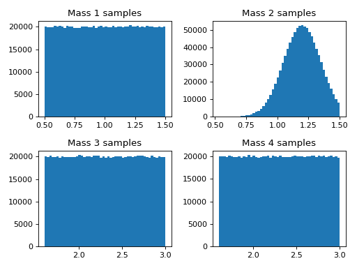
Making Mass Distributions in M1 and M2
Here we will demonstrate how to make different mass populations of binaries. This example shows uniform and gaussian mass distributions.
import matplotlib.pyplot as plt
from pycbc import distributions

# Create a mass distribution object that is uniform between 0.5 and 1.5
# solar masses.
mass1_distribution = distributions.Uniform(mass1=(0.5, 1.5))
# Take 100000 random variable samples from this uniform mass distribution.
mass1_samples = mass1_distribution.rvs(size=1000000)

# Draw another distribution that is Gaussian between 0.5 and 1.5 solar masses
# with a mean of 1.2 solar masses and a standard deviation of 0.15 solar
# masses. Gaussian takes the variance as an input so square the standard
# deviation.
variance = 0.15*0.15
mass2_gaussian = distributions.Gaussian(mass2=(0.5, 1.5), mass2_mean=1.2,
                                        mass2_var=variance)

# Take 100000 random variable samples from this gaussian mass distribution.
mass2_samples = mass2_gaussian.rvs(size=1000000)

# We can make pairs of distributions together, instead of apart.
two_mass_distributions = distributions.Uniform(mass3=(1.6, 3.0),
                                               mass4=(1.6, 3.0))
two_mass_samples = two_mass_distributions.rvs(size=1000000)

# Choose 50 bins for the histogram subplots.
n_bins = 50

# Plot histograms of samples in subplots
fig, axes = plt.subplots(nrows=2, ncols=2)
ax0, ax1, ax2, ax3, = axes.flat

ax0.hist(mass1_samples['mass1'], bins = n_bins)
ax1.hist(mass2_samples['mass2'], bins = n_bins)
ax2.hist(two_mass_samples['mass3'], bins = n_bins)
ax3.hist(two_mass_samples['mass4'], bins = n_bins)

ax0.set_title('Mass 1 samples')
ax1.set_title('Mass 2 samples')
ax2.set_title('Mass 3 samples')
ax3.set_title('Mass 4 samples')

plt.tight_layout()
plt.show()
(Source code, png, hires.png, pdf)
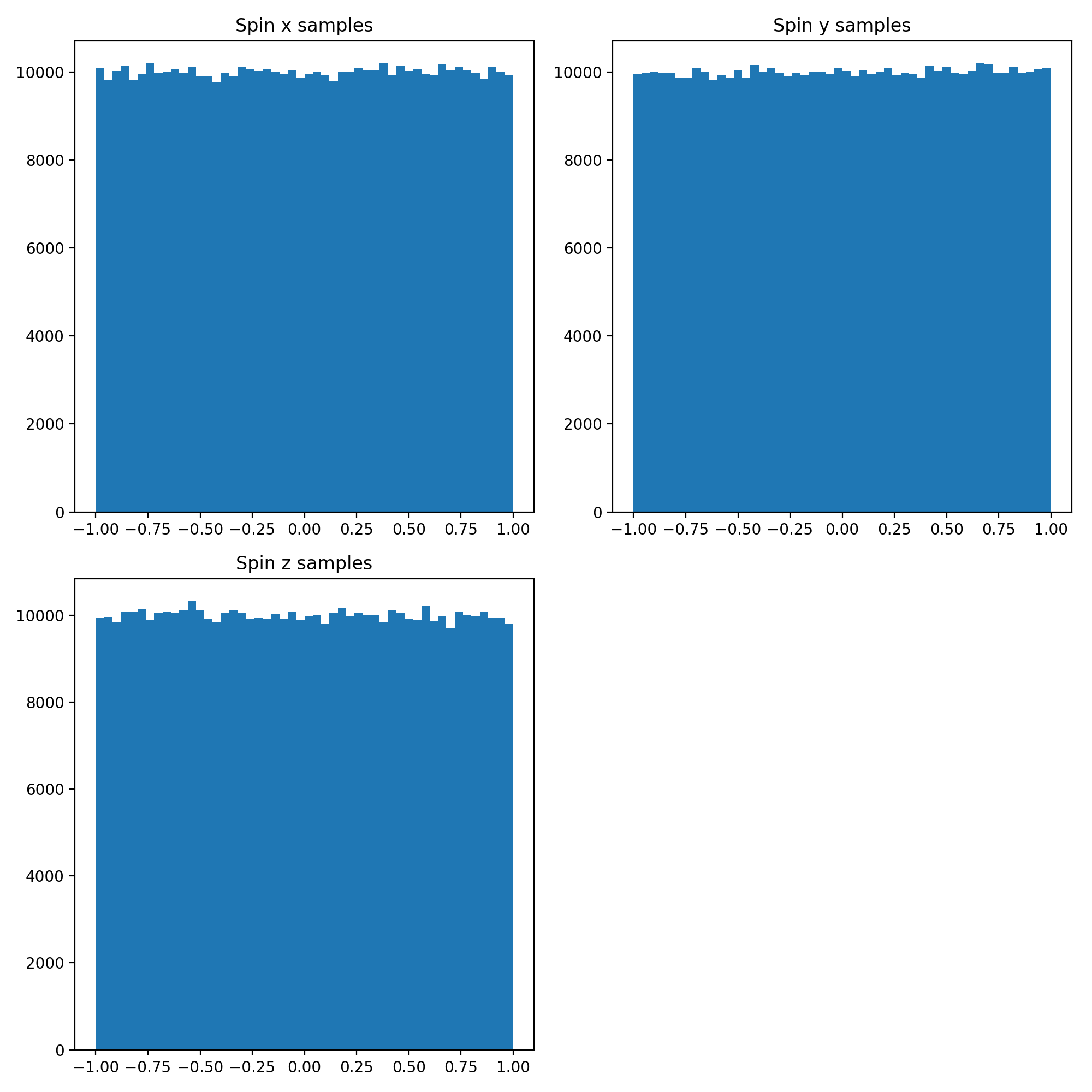
Sky Location Distribution as Spin Distribution Example
Here we can make a distribution of spins of unit length with equal distribution in x, y, and z to sample the surface of a unit sphere.
import matplotlib.pyplot as plt
import numpy
import pycbc.coordinates as co
from pycbc import distributions

# We can choose any bounds between 0 and pi for this distribution but in
# units of pi so we use between 0 and 1
theta_low = 0.
theta_high = 1.

# Units of pi for the bounds of the azimuthal angle which goes from 0 to 2 pi
phi_low = 0.
phi_high = 2.

# Create a distribution object from distributions.py. Here we are using the
# Uniform Solid Angle function which takes
# theta = polar_bounds(theta_lower_bound to a theta_upper_bound), and then
# phi = azimuthal_ bound(phi_lower_bound to a phi_upper_bound).
uniform_solid_angle_distribution = distributions.UniformSolidAngle(
                                          polar_bounds=(theta_low,theta_high),
                                          azimuthal_bounds=(phi_low,phi_high))

# Now we can take a random variable sample from that distribution. In this
# case we want 50000 samples.
solid_angle_samples = uniform_solid_angle_distribution.rvs(size=500000)

# Make spins with unit length for coordinate transformation below.
spin_mag = numpy.ndarray(shape=(500000), dtype=float)

for i in range(0,500000):
    spin_mag[i] = 1.

# Use the pycbc.coordinates as co spherical_to_cartesian function to convert
# from spherical polar coordinates to cartesian coordinates
spinx, spiny, spinz = co.spherical_to_cartesian(spin_mag,
                                                solid_angle_samples['phi'],
                                                solid_angle_samples['theta'])

# Choose 50 bins for the histograms.
n_bins = 50

plt.figure(figsize=(10,10))
plt.subplot(2, 2, 1)
plt.hist(spinx, bins = n_bins)
plt.title('Spin x samples')

plt.subplot(2, 2, 2)
plt.hist(spiny, bins = n_bins)
plt.title('Spin y samples')

plt.subplot(2, 2, 3)
plt.hist(spinz, bins = n_bins)
plt.title('Spin z samples')

plt.tight_layout()
plt.show()
(Source code, png, hires.png, pdf)

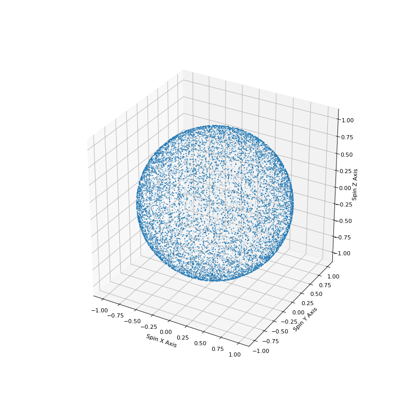
Using much of the same code we can also show how this sampling accurately covers the surface of a unit sphere.
import numpy
import matplotlib.pyplot as plt
import pycbc.coordinates as co
from mpl_toolkits.mplot3d import Axes3D
from pycbc import distributions

# We can choose any bounds between 0 and pi for this distribution but in units
# of pi so we use between 0 and 1.
theta_low = 0.
theta_high = 1.

# Units of pi for the bounds of the azimuthal angle which goes from 0 to 2 pi.
phi_low = 0.
phi_high = 2.

# Create a distribution object from distributions.py
# Here we are using the Uniform Solid Angle function which takes
# theta = polar_bounds(theta_lower_bound to a theta_upper_bound), and then
# phi = azimuthal_bound(phi_lower_bound to a phi_upper_bound).
uniform_solid_angle_distribution = distributions.UniformSolidAngle(
                                          polar_bounds=(theta_low,theta_high),
                                          azimuthal_bounds=(phi_low,phi_high))

# Now we can take a random variable sample from that distribution.
# In this case we want 50000 samples.
solid_angle_samples = uniform_solid_angle_distribution.rvs(size=10000)

# Make a spin 1 magnitude since solid angle is only 2 dimensions and we need a
# 3rd dimension for a 3D plot that we make later on.
spin_mag = numpy.ndarray(shape=(10000), dtype=float)

for i in range(0,10000):
    spin_mag[i] = 1.

# Use pycbc.coordinates as co. Use  spherical_to_cartesian function to
# convert from spherical polar coordinates to cartesian coordinates.
spinx, spiny, spinz = co.spherical_to_cartesian(spin_mag,
                                                solid_angle_samples['phi'],
                                                solid_angle_samples['theta'])

# Plot the spherical distribution of spins to make sure that we
# distributed across  the surface of a sphere.

fig = plt.figure(figsize=(10,10))
ax = fig.add_subplot(111, projection='3d')
ax.scatter(spinx, spiny, spinz, s=1)

ax.set_xlabel('Spin X Axis')
ax.set_ylabel('Spin Y Axis')
ax.set_zlabel('Spin Z Axis')
plt.show()
(Source code, png, hires.png, pdf)