PyCBC inference documentation (pycbc.inference)
Introduction
This page gives details on how to use the various parameter estimation
executables and modules available in PyCBC. The pycbc.inference subpackage
contains classes and functions for evaluating probability distributions,
likelihoods, and running Bayesian samplers.
Sampling the parameter space (pycbc_inference)
Overview
The executable pycbc_inference is designed to sample the parameter space
and save the samples in an HDF file. A high-level description of the
pycbc_inference algorithm is
Read priors from a configuration file.
Setup the model to use. If the model uses data, then:
- Read gravitational-wave strain from a gravitational-wave model or use recolored fake strain.
- Estimate a PSD.
Run a sampler to estimate the posterior distribution of the model.
Write the samples and metadata to an HDF file.
The model, data, sampler, parameters to vary and their priors are specified in
one or more configuration files, which are passed to the program using the
--config-file option. Other command-line options determine what
parallelization settings to use. For a full listing of all options run
pycbc_inference --help. Below, we give details on how to set up a
configuration file and provide examples of how to run pycbc_inference.
Configuring the model, sampler, priors, and data
The configuration file(s) uses WorkflowConfigParser syntax. The required
sections are: [model], [sampler], and [variable_params]. In
addition, multiple [prior] sections must be provided that define the prior
distribution to use for the parameters in [variable_params]. If a model
uses data a [data] section must also be provided.
These sections may be split up over multiple files. In that case, all of the
files should be provided as space-separated arguments to the --config-file.
Providing multiple files is equivalent to providing a single file with
everything across the files combined. If the same section is specified in
multiple files, the all of the options will be combined.
Configuration files allow for referencing values in other sections using the
syntax ${section|option}. See the examples below for an example of this.
When providing multiple configuration files, sections in other files may be
referenced, since in the multiple files are combined into a single file in
memory when the files are loaded.
Configuring the model
The [model] section sets up what model to use for the analysis. At minimum,
a name argument must be provided, specifying which model to use. For
example:
[model]
name = gaussian_noise
In this case, the GaussianNoise model would be used. (Examples of using this
model on a BBH injection and on GW150914 are given below.) Other arguments to
configure the model may also be set in this section. The recognized arguments
depend on the model. The currently available models are:
| Name | Class |
|---|---|
'gaussian_noise' |
pycbc.inference.models.gaussian_noise.GaussianNoise |
'marginalized_gaussian_noise' |
pycbc.inference.models.marginalized_gaussian_noise.MarginalizedGaussianNoise |
'marginalized_phase' |
pycbc.inference.models.marginalized_gaussian_noise.MarginalizedPhaseGaussianNoise |
'single_template' |
pycbc.inference.models.single_template.SingleTemplate |
'test_eggbox' |
pycbc.inference.models.analytic.TestEggbox |
'test_normal' |
pycbc.inference.models.analytic.TestNormal |
'test_prior' |
pycbc.inference.models.analytic.TestPrior |
'test_rosenbrock' |
pycbc.inference.models.analytic.TestRosenbrock |
'test_volcano' |
pycbc.inference.models.analytic.TestVolcano |
Refer to the models’ from_config method to see what configuration arguments
are available.
Any model name that starts with test_ is an analytic test distribution that
requires no data or waveform generation. See the section below on running on an
analytic distribution for more details.
Configuring the sampler
The [sampler] section sets up what sampler to use for the analysis. As
with the [model] section, a name must be provided to specify which
sampler to use. The currently available samplers are:
| Name | Class |
|---|---|
'dynesty' |
pycbc.inference.sampler.dynesty.DynestySampler |
'emcee' |
pycbc.inference.sampler.emcee.EmceeEnsembleSampler |
'emcee_pt' |
pycbc.inference.sampler.emcee_pt.EmceePTSampler |
'multinest' |
pycbc.inference.sampler.multinest.MultinestSampler |
Configuration options for the sampler should also be specified in the
[sampler] section. For example:
[sampler]
name = emcee
nwalkers = 5000
niterations = 1000
checkpoint-interval = 100
This would tell pycbc_inference to run the
EmceeEnsembleSampler
with 5000 walkers for 1000 iterations, checkpointing every 100th iteration.
Refer to the samplers’ from_config method to see what configuration options
are available.
Burn-in tests may also be configured for MCMC samplers in the config file. The
options for the burn-in should be placed in [sampler-burn_in]. At minimum,
a burn-in-test argument must be given in this section. This argument
specifies which test(s) to apply. Multiple tests may be combined using standard
python logic operators. For example:
[sampler-burn_in]
burn-in-test = nacl & max_posterior
In this case, the sampler would be considered to be burned in when both the
nacl and max_posterior tests were satisfied. Setting this to nacl |
max_postrior would instead consider the sampler to be burned in when either
the nacl or max_posterior tests were satisfied. For more information
on what tests are available, see the pycbc.inference.burn_in module.
Thinning samples (MCMC only)
The default behavior for the MCMC samplers (emcee, emcee_pt) is to save
every iteration of the Markov chains to the output file. This can quickly lead
to very large files. For example, a BBH analysis (~15 parameters) with 200
walkers, 20 temperatures may take ~50 000 iterations to acquire ~5000
independent samples. This will lead to a file that is ~ 50 000 iterations x 200
walkers x 20 temperatures x 15 parameters x 8 bytes ~ 20GB. Quieter signals
can take an order of magnitude more iterations to converge, leading to O(100GB)
files. Clearly, since we only obtain 5000 independent samples from such a run,
the vast majority of these samples are of little interest.
To prevent large file size growth, samples may be thinned before they are
written to disk. Two thinning options are available, both of which are set in
the [sampler] section of the configuration file. They are:
thin-interval: This will thin the samples by the given integer before writing the samples to disk. File sizes can still grow unbounded, but at a slower rate. The interval must be less than the checkpoint interval.max-samples-per-chain: This will cap the maximum number of samples per walker and per temperature to the given integer. This ensures that file sizes never exceed ~max-samples-per-chainxnwalkersxntempsxnparametersx 8 bytes. Once the limit is reached, samples will be thinned on disk, and new samples will be thinned to match. The thinning interval will grow with longer runs as a result. To ensure that enough samples exist to determine burn in and to measure an autocorrelation length,max-samples-per-chainmust be greater than or equal to 100.
The thinned interval that was used for thinning samples is saved to the output
file’s thinned_by attribute (stored in the HDF file’s .attrs). Note
that this is not the autocorrelation length (ACL), which is the amount that the
samples need to be further thinned to obtain independent samples.
Note
In the output file creates by the MCMC samplers, we adopt the convention
that “iteration” means iteration of the sampler, not index of the samples.
For example, if a burn in test is used, burn_in_iteration will be
stored to the sampler_info group in the output file. This gives the
iteration of the sampler at which burn in occurred, not the sample on disk.
To determine which samples an iteration corresponds to in the file, divide
iteration by thinned_by.
Likewise, we adopt the convention that autocorrelation length (ACL) is
the autocorrelation length of the thinned samples (the number of samples on
disk that you need to skip to get independent samples) whereas
autocorrelation time (ACT) is the autocorrelation length in terms of
iteration (it is the number of iterations that you need to skip to get
independent samples); i.e., ACT = thinned_by x ACL. The ACT is (up to
measurement resolution) independent of the thinning used, and thus is
useful for comparing the performance of the sampler.
Configuring the prior
What parameters to vary to obtain a posterior distribution are determined by
[variable_params] section. For example:
[variable_params]
x =
y =
This would tell pycbc_inference to sample a posterior over two parameters
called x and y.
A prior must be provided for every parameter in [variable_params]. This
is done by adding sections named [prior-{param}] where {param} is the
name of the parameter the prior is for. For example, to provide a prior for the
x parameter in the above example, you would need to add a section called
[prior-x]. If the prior couples more than one parameter together in a joint
distribution, the parameters should be provided as a + separated list,
e.g., [prior-x+y+z].
The prior sections specify what distribution to use for the parameter’s prior,
along with any settings for that distribution. Similar to the model and
sampler sections, each prior section must have a name argument that
identifies the distribution to use. Distributions are defined in the
pycbc.distributions module. The currently available distributions
are:
| Name | Class |
|---|---|
'arbitrary' |
pycbc.distributions.arbitrary.Arbitrary |
'cos_angle' |
pycbc.distributions.angular.CosAngle |
'fromfile' |
pycbc.distributions.arbitrary.FromFile |
'gaussian' |
pycbc.distributions.gaussian.Gaussian |
'independent_chip_chieff' |
pycbc.distributions.spins.IndependentChiPChiEff |
'sin_angle' |
pycbc.distributions.angular.SinAngle |
'uniform' |
pycbc.distributions.uniform.Uniform |
'uniform_angle' |
pycbc.distributions.angular.UniformAngle |
'uniform_f0_tau' |
pycbc.distributions.qnm.UniformF0Tau |
'uniform_log10' |
pycbc.distributions.uniform_log.UniformLog10 |
'uniform_power_law' |
pycbc.distributions.power_law.UniformPowerLaw |
'uniform_radius' |
pycbc.distributions.power_law.UniformRadius |
'uniform_sky' |
pycbc.distributions.sky_location.UniformSky |
'uniform_solidangle' |
pycbc.distributions.angular.UniformSolidAngle |
Static parameters
A [static_params] section may be provided to list any parameters that
will remain fixed throughout the run. For example:
[static_params]
approximant = IMRPhenomPv2
f_lower = 18
Setting data
Many models, such as the GaussianNoise model, require data to be provided. To
do so, a [data] section must be included that provides information about
what data to load, and how to condition it.
The type of data to be loaded depends on the model. For example, if you are
using the GaussianNoise or MarginalizedPhaseGaussianNoise models (the
typical case), one will need to load gravitational-wave data. This is
accomplished using tools provided in the pycbc.strain module. The
full set of options are:
| Name | Syntax | Description |
|---|---|---|
instruments |
INSTRUMENTS [INSTRUMENTS …] | Instruments to analyze, eg. H1 L1. |
trigger-time |
TRIGGER_TIME | Reference GPS time (at geocenter) from which the (anlaysis|psd)-(start|end)-time options are measured. The integer seconds will be used. Default is 0; i.e., if not provided, the analysis and psd times should be in GPS seconds. |
analysis-start-time |
IFO:TIME [IFO:TIME …] | The start time to use for the analysis, measured with respect to the trigger-time. If psd-inverse-length is provided, the given start time will be padded by half that length to account for wrap-around effects. |
analysis-end-time |
IFO:TIME [IFO:TIME …] | The end time to use for the analysis, measured with respect to the trigger-time. If psd-inverse-length is provided, the given end time will be padded by half that length to account for wrap-around effects. |
psd-start-time |
IFO:TIME [IFO:TIME …] | Start time to use for PSD estimation, measured with respect to the trigger-time. |
psd-end-time |
IFO:TIME [IFO:TIME …] | End time to use for PSD estimation, measured with respect to the trigger-time. |
data-conditioning-low-freq |
IFO:FLOW [IFO:FLOW …] | Low frequency cutoff of the data. Needed for PSD estimation and when creating fake strain. If not provided, will use the model’s low-frequency-cutoff. |
Options to select the method of PSD generation:
The options psd-model, psd-file, asd-file, and psd-estimation are
mutually exclusive. |
||
psd-model |
IFO:MODEL [IFO:MODEL …] | Get PSD from given analytical model. Choose from any available PSD model. |
psd-file |
IFO:FILE [IFO:FILE …] | Get PSD using given PSD ASCII file |
asd-file |
IFO:FILE [IFO:FILE …] | Get PSD using given ASD ASCII file |
psd-estimation |
IFO:FILE [IFO:FILE …] | Measure PSD from the data, using given average method. Choose from mean, median or median-mean. |
psd-segment-length |
IFO:LENGTH [IFO:LENGTH …] | (Required for psd-estimation) The segment length for
PSD estimation (s) |
psd-segment-stride |
IFO:STRIDE [IFO:STRIDE …] | (Required for psd-estimation) The separation between
consecutive segments (s) |
psd-num-segments |
IFO:NUM [IFO:NUM …] | (Optional, used only with psd-estimation). If given
PSDs will be estimated using only this number of
segments. If more data is given than needed to make
this number of segments than excess data will not be
used in the PSD estimate. If not enough data is given
the code will fail. |
psd-inverse-length |
IFO:LENGTH [IFO:LENGTH …] | (Optional) The maximum length of the impulse response of the overwhitening filter (s) |
psd-output |
IFO:FILE [IFO:FILE …] | (Optional) Write PSD to specified file |
psdvar-segment |
SECONDS | Length of segment when calculating the PSD variability. |
psdvar-short-segment |
SECONDS | Length of short segment for outliers removal in PSD variability calculation. |
psdvar-long-segment |
SECONDS | Length of long segment when calculating the PSD variability. |
psdvar-psd-duration |
SECONDS | Duration of short segments for PSD estimation. |
psdvar-psd-stride |
SECONDS | Separation between PSD estimation segments. |
psdvar-low-freq |
HERTZ | Minimum frequency to consider in strain bandpass. |
psdvar-high-freq |
HERTZ | Maximum frequency to consider in strain bandpass. |
Options for obtaining h(t):
These options are used for generating h(t) either by reading from a file
or by generating it. This is only needed if the PSD is to be estimated
from the data, ie. if the psd-estimation option is given. This group
supports reading from multiple ifos simultaneously. |
||
strain-high-pass |
IFO:FREQUENCY [IFO:FREQUENCY …] | High pass frequency |
pad-data |
IFO:LENGTH [IFO:LENGTH …] | Extra padding to remove highpass corruption (integer seconds) |
taper-data |
IFO:LENGTH [IFO:LENGTH …] | Taper ends of data to zero using the supplied length as a window (integer seconds) |
sample-rate |
IFO:RATE [IFO:RATE …] | The sample rate to use for h(t) generation (integer Hz). |
channel-name |
IFO:CHANNEL [IFO:CHANNEL …] | The channel containing the gravitational strain data |
frame-cache |
IFO:FRAME_CACHE [IFO:FRAME_CACHE …] | Cache file containing the frame locations. |
frame-files |
IFO:FRAME_FILES [IFO:FRAME_FILES …] | list of frame files |
hdf-store |
IFO:HDF_STORE_FILE [IFO:HDF_STORE_FILE …] | Store of time series data in hdf format |
frame-type |
IFO:FRAME_TYPE [IFO:FRAME_TYPE …] | (optional) Replaces frame-files. Use datafind to get the needed frame file(s) of this type. |
frame-sieve |
IFO:FRAME_SIEVE [IFO:FRAME_SIEVE …] | (optional), Only use frame files where the URL matches the regular expression given. |
fake-strain |
IFO:CHOICE [IFO:CHOICE …] | Name of model PSD for generating fake gaussian noise.
Choose from any available PSD model, or zeroNoise. |
fake-strain-seed |
IFO:SEED [IFO:SEED …] | Seed value for the generation of fake colored gaussian noise |
fake-strain-from-file |
IFO:FILE [IFO:FILE …] | File containing ASD for generating fake noise from it. |
injection-file |
IFO:FILE [IFO:FILE …] | (optional) Injection file used to add waveforms into the strain |
sgburst-injection-file |
IFO:FILE [IFO:FILE …] | (optional) Injection file used to add sine-Gaussian burst waveforms into the strain |
injection-scale-factor |
IFO:VAL [IFO:VAL …] | Multiple injections by this factor before injecting into the data. |
injection-f-ref |
IFO:VALUE | Reference frequency in Hz for creating CBC injections from an XML file. |
injection-f-final |
IFO:VALUE | Override the f_final field of a CBC XML injection file. |
gating-file |
IFO:FILE [IFO:FILE …] | (optional) Text file of gating segments to apply. Format of each line (units s) : gps_time zeros_half_width pad_half_width |
autogating-threshold |
IFO:SIGMA [IFO:SIGMA …] | If given, find and gate glitches producing a deviation larger than SIGMA in the whitened strain time series. |
autogating-max-iterations |
SIGMA | If given, iteratively apply autogating |
autogating-cluster |
IFO:SECONDS [IFO:SECONDS …] | Length of clustering window for detecting glitches for autogating. |
autogating-width |
IFO:SECONDS [IFO:SECONDS …] | Half-width of the gating window. |
autogating-taper |
IFO:SECONDS [IFO:SECONDS …] | Taper the strain before and after each gating window over a duration of SECONDS. |
autogating-pad |
IFO:SECONDS [IFO:SECONDS …] | Ignore the given length of whitened strain at the ends of a segment, to avoid filters ringing. |
normalize-strain |
IFO:VALUE [IFO:VALUE …] | (optional) Divide frame data by constant. |
zpk-z |
IFO:VALUE [IFO:VALUE …] | (optional) Zero-pole-gain (zpk) filter strain. A list of zeros for transfer function |
zpk-p |
IFO:VALUE [IFO:VALUE …] | (optional) Zero-pole-gain (zpk) filter strain. A list of poles for transfer function |
zpk-k |
IFO:VALUE [IFO:VALUE …] | (optional) Zero-pole-gain (zpk) filter strain. Transfer function gain |
| Options for gating data: | ||
gate |
IFO:CENTRALTIME:HALFDUR:TAPERDUR [IFO:CENTRALTIME:HALFDUR:TAPERDUR …] | Apply one or more gates to the data before filtering. |
gate-overwhitened |
Overwhiten data first, then apply the gates specified
in gate. Overwhitening allows for sharper tapers to
be used, since lines are not blurred. |
|
psd-gate |
IFO:CENTRALTIME:HALFDUR:TAPERDUR [IFO:CENTRALTIME:HALFDUR:TAPERDUR …] | Apply one or more gates to the data used for computing the PSD. Gates are applied prior to FFT-ing the data for PSD estimation. |
| Options for quering data quality (DQ): | ||
dq-segment-name |
DQ_SEGMENT_NAME | The status flag to query for data quality. Default is “DATA”. |
dq-source |
{any,GWOSC,dqsegdb} | Where to look for DQ information. If “any” (the default) will first try GWOSC, then dqsegdb. |
dq-server |
DQ_SERVER | The server to use for dqsegdb. |
veto-definer |
VETO_DEFINER | Path to a veto definer file that defines groups of flags, which themselves define a set of DQ segments. |
As indicated in the table, the psd-model and fake-strain options can
accept an analytical PSD as an argument. The available PSD models are:
Advanced configuration settings
The following are additional settings that may be provided in the configuration file, in order to do more sophisticated analyses.
Sampling transforms
One or more of the variable_params may be transformed to a different
parameter space for purposes of sampling. This is done by specifying a
[sampling_params] section. This section specifies which
variable_params to replace with which parameters for sampling. This must be
followed by one or more [sampling_transforms-{sampling_params}] sections
that provide the transform class to use. For example, the following would cause
the sampler to sample in chirp mass (mchirp) and mass ratio (q) instead
of mass1 and mass2:
[sampling_params]
mass1, mass2: mchirp, q

[sampling_transforms-mchirp+q]
name = mass1_mass2_to_mchirp_q
Transforms are provided by the pycbc.transforms module. The currently
available transforms are:
Note
Both a jacobian and inverse_jacobian must be defined in order to use
a transform class for a sampling transform. Not all transform classes in
pycbc.transforms have these defined. Check the class
documentation to see if a Jacobian is defined.
Waveform transforms
There can be any number of variable_params with any name. No parameter name
is special (with the exception of parameters that start with calib_; see
below).
However, when doing parameter estimation with CBC waveforms, certain parameter names must be provided for waveform generation. The parameter names recognized by the CBC waveform generators are:
| Parameter | Description |
|---|---|
'mass1' |
The mass of the first component object in the binary (in solar masses). |
'mass2' |
The mass of the second component object in the binary (in solar masses). |
'spin1x' |
The x component of the first binary component’s dimensionless spin. |
'spin1y' |
The y component of the first binary component’s dimensionless spin. |
'spin1z' |
The z component of the first binary component’s dimensionless spin. |
'spin2x' |
The x component of the second binary component’s dimensionless spin. |
'spin2y' |
The y component of the second binary component’s dimensionless spin. |
'spin2z' |
The z component of the second binary component’s dimensionless spin. |
'eccentricity' |
Eccentricity. |
'lambda1' |
The dimensionless tidal deformability parameter of object 1. |
'lambda2' |
The dimensionless tidal deformability parameter of object 2. |
'dquad_mon1' |
Quadrupole-monopole parameter / m_1^5 -1. |
'dquad_mon2' |
Quadrupole-monopole parameter / m_2^5 -1. |
'lambda_octu1' |
The octupolar tidal deformability parameter of object 1. |
'lambda_octu2' |
The octupolar tidal deformability parameter of object 2. |
'quadfmode1' |
The quadrupolar f-mode angular frequency of object 1. |
'quadfmode2' |
The quadrupolar f-mode angular frequency of object 2. |
'octufmode1' |
The octupolar f-mode angular frequency of object 1. |
'octufmode2' |
The octupolar f-mode angular frequency of object 2. |
'distance' |
Luminosity distance to the binary (in Mpc). |
'coa_phase' |
Coalesence phase of the binary (in rad). |
'inclination' |
Inclination (rad), defined as the angle between the total angular momentum J and the line-of-sight. |
'long_asc_nodes' |
Longitude of ascending nodes axis (rad). |
'mean_per_ano' |
Mean anomaly of the periastron (rad). |
'delta_t' |
The time step used to generate the waveform (in s). |
'f_lower' |
The starting frequency of the waveform (in Hz). |
'approximant' |
A string that indicates the chosen approximant. |
'f_ref' |
The reference frequency. |
'phase_order' |
The pN order of the orbital phase. The default of -1 indicates that all implemented orders are used. |
'spin_order' |
The pN order of the spin corrections. The default of -1 indicates that all implemented orders are used. |
'tidal_order' |
The pN order of the tidal corrections. The default of -1 indicates that all implemented orders are used. |
'amplitude_order' |
The pN order of the amplitude. The default of -1 indicates that all implemented orders are used. |
'eccentricity_order' |
The pN order of the eccentricity corrections.The default of -1 indicates that all implemented orders are used. |
'frame_axis' |
Allow to choose among orbital_l, view and total_j |
'modes_choice' |
Allow to turn on among orbital_l, view and total_j |
'side_bands' |
Flag for generating sidebands |
'mode_array' |
Choose which (l,m) modes to include when generating a waveform. Only if approximant supports this feature.By default pass None and let lalsimulation use it’s default behaviour.Example: mode_array = [ [2,2], [2,-2] ] |
'numrel_data' |
Sets the NR flags; only needed for NR waveforms. |
'delta_f' |
The frequency step used to generate the waveform (in Hz). |
'f_final' |
The ending frequency of the waveform. The default (0) indicates that the choice is made by the respective approximant. |
'f_final_func' |
Use the given frequency function to compute f_final based on the parameters of the waveform. |
'tc' |
Coalescence time (s). |
'ra' |
Right ascension (rad). |
'dec' |
Declination (rad). |
'polarization' |
Polarization (rad). |
It is possible to specify a variable_param that is not one of these
parameters. To do so, you must provide one or more
[waveforms_transforms-{param}] section(s) that define transform(s) from the
arbitrary variable_params to the needed waveform parameter(s) {param}.
For example, in the following we provide a prior on chirp_distance. Since
distance, not chirp_distance, is recognized by the CBC waveforms
module, we provide a transform to go from chirp_distance to distance:
[variable_params]
chirp_distance =

[prior-chirp_distance]
name = uniform
min-chirp_distance = 1
max-chirp_distance = 200

[waveform_transforms-distance]
name = chirp_distance_to_distance
A useful transform for these purposes is the
CustomTransform, which allows
for arbitrary transforms using any function in the pycbc.conversions,
pycbc.coordinates, or pycbc.cosmology modules, along with
numpy math functions. For example, the following would use the I-Love-Q
relationship pycbc.conversions.dquadmon_from_lambda() to relate the
quadrupole moment of a neutron star dquad_mon1 to its tidal deformation
lambda1:
[variable_params]
lambda1 =

[waveform_transforms-dquad_mon1]
name = custom
inputs = lambda1
dquad_mon1 = dquadmon_from_lambda(lambda1)
Note
A Jacobian is not necessary for waveform transforms, since the transforms are only being used to convert a set of parameters into something that the waveform generator understands. This is why in the above example we are able to use a custom transform without needing to provide a Jacobian.
Some common transforms are pre-defined in the code. These are: the mass
parameters mass1 and mass2 can be substituted with mchirp and
eta or mchirp and q. The component spin parameters spin1x,
spin1y, and spin1z can be substituted for polar coordinates
spin1_a, spin1_azimuthal, and spin1_polar (ditto for spin2).
Calibration parameters
If any calibration parameters are used (prefix calib_), a [calibration]
section must be included. This section must have a name option that
identifies what calibration model to use. The models are described in
pycbc.calibration. The [calibration] section must also include
reference values fc0, fs0, and qinv0, as well as paths to ASCII
transfer function files for the test mass actuation, penultimate mass
actuation, sensing function, and digital filter for each IFO being used in the
analysis. E.g. for an analysis using H1 only, the required options would be
h1-fc0, h1-fs0, h1-qinv0, h1-transfer-function-a-tst,
h1-transfer-function-a-pu, h1-transfer-function-c,
h1-transfer-function-d.
Constraints
One or more constraints may be applied to the parameters; these are
specified by the [constraint] section(s). Additional constraints may be
supplied by adding more [constraint-{tag}] sections. Any tag may be used; the
only requirement is that they be unique. If multiple constraint sections are
provided, the union of all constraints is applied. Alternatively, multiple
constraints may be joined in a single argument using numpy’s logical operators.
The parameter that constraints are applied to may be any parameter in
variable_params or any output parameter of the transforms. Functions may be
applied to these parameters to obtain constraints on derived parameters. Any
function in the conversions, coordinates, or cosmology module may be used,
along with any numpy ufunc. So, in the following example, the mass ratio (q) is
constrained to be <= 4 by using a function from the conversions module.
[variable_params]
mass1 =
mass2 =

[prior-mass1]
name = uniform
min-mass1 = 3
max-mass1 = 12

[prior-mass2]
name = uniform
min-mass2 = 1
min-mass2 = 3

[constraint-1]
name = custom
constraint_arg = q_from_mass1_mass2(mass1, mass2) <= 4
Checkpointing and output files
While pycbc_inference is running it will create a checkpoint file which
is named {output-file}.checkpoint, where {output-file} was the name
of the file you specified with the --output-file command. When it
checkpoints it will dump results to this file; when finished, the file is
renamed to {output-file}. A {output-file}.bkup is also created, which
is a copy of the checkpoint file. This is kept in case the checkpoint file gets
corrupted during writing. The .bkup file is deleted at the end of the run,
unless --save-backup is turned on.
When pycbc_inference starts, it checks if either
{output-file}.checkpoint or {output-file}.bkup exist (in that order).
If at least one of them exists, pycbc_inference will attempt to load them
and continue to run from the last checkpoint state they were in.
The output/checkpoint file are HDF files. To peruse the structure of the file
you can use the h5ls command-line utility. More advanced utilities for
reading and writing from/to them are provided by the sampler IO classes in
pycbc.inference.io. To load one of these files in python do:
from pycbc.inference import io
fp = io.loadfile(filename, "r")
Here, fp is an instance of a sampler IO class. Basically, this is an
instance of an h5py.File handler, with additional
convenience functions added on top. For example, if you want all of the samples
of all of the variable parameters in the file, you can do:
samples = fp.read_samples(fp.variable_params)
This will return a FieldArray of all
of the samples.
Each sampler has it’s own sampler IO class that adds different convenience
functions, depending on the sampler that was used. For more details on these
classes, see the pycbc.inference.io module.
Examples
Examples are given in the subsections below.
Running on an analytic distribution
Several analytic distributions are available to run tests on. These can be run quickly on a laptop to check that a sampler is working properly.
This example demonstrates how to sample a 2D normal distribution with the
emcee sampler. First, we create the following configuration file:
[model]
name = test_normal

[sampler]
name = emcee
nwalkers = 5000
niterations = 100

[variable_params]
x =
y =

[prior-x]
name = uniform
min-x = -10
max-x = 10

[prior-y]
name = uniform
min-y = -10
max-y = 10
By setting the model name to test_normal we are using
TestNormal.
The number of dimensions of the distribution is set by the number of
variable_params. The names of the parameters do not matter, just that just
that the prior sections use the same names.
Now run:
#!/bin/sh
pycbc_inference --verbose \
        --config-files normal2d.ini \
        --output-file normal2d.hdf \
        --nprocesses 2 \
        --seed 10 \
        --force
This will run the emcee sampler on the 2D analytic normal distribution with
5000 walkers for 100 iterations. When it is done, you will have a file called
normal2d.hdf which contains the results. It should take about a minute to
run. If you have a computer with more cores, you can increase the
parallelization by changing the nprocesses argument.
To plot the posterior distribution after the last iteration, run:
#!/bin/sh
pycbc_inference_plot_posterior --verbose \
        --input-file normal2d.hdf \
        --output-file posterior-normal2d.png \
        --plot-scatter \
        --plot-contours \
        --plot-marginal \
        --z-arg 'loglikelihood:$\log p(h|\vartheta)$' \
        --iteration -1
This will create the following plot:
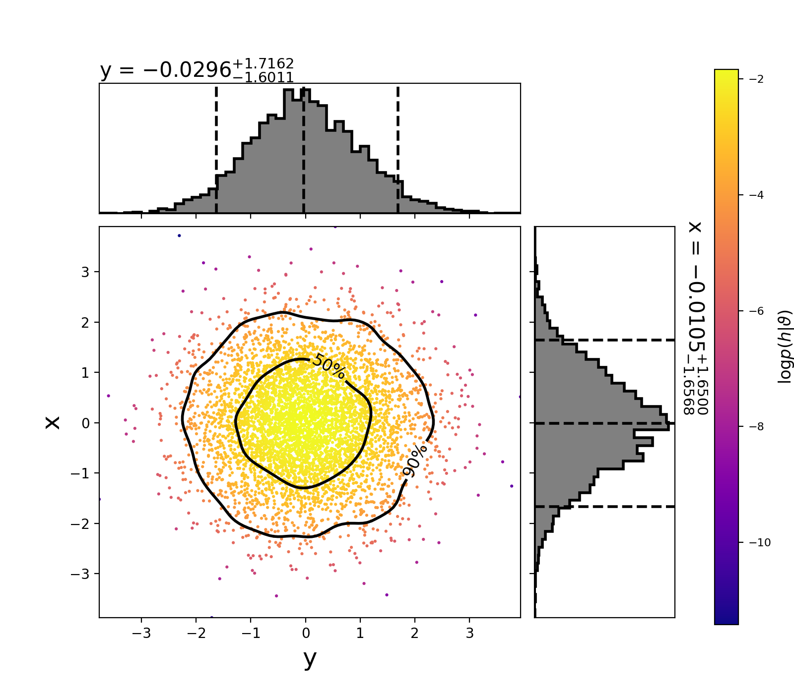
The scatter points show each walker’s position after the last iteration. The points are colored by the log likelihood at that point, with the 50th and 90th percentile contours drawn.
See below for more information about using pycbc_inference_plot_posterior.
To make a movie showing how the walkers evolved, run:
#!/bin/sh
pycbc_inference_plot_movie --verbose \
        --nprocesses 4 \
        --input-file normal2d.hdf \
        --output-prefix frames-normal2d \
        --movie-file normal2d_mcmc_evolution.mp4 \
        --cleanup \
        --plot-scatter \
        --plot-contours \
        --plot-marginal \
        --z-arg 'loglikelihood:$\log p(h|\vartheta)$' \
        --frame-step 1
Note
You need ffmpeg installed for the mp4 to be created.
See below for more information on using pycbc_inference_plot_movie.
Simulated BBH example
This example recovers the parameters of a simulated binary black-hole (BBH) that has similar parameters has GW150914.
Creating the injection
First, we need to create an injection.hdf file that specifies the
parameters of the simulated signal. To do that we will use
pycbc_create_injection. Like pycbc_inference,
pycbc_create_injections uses a configuration file to set the parameters of
the injections it will create. To create a binary-black hole with parameters
similar to GW150914, use the following configuration file:
[variable_params]

[static_params]
tc = 1126259462.420
mass1 = 37
mass2 = 32
ra = 2.2
dec = -1.25
inclincation = 2.5
coa_phase = 1.5
polarization = 1.75
distance = 100
f_ref = 20
f_lower = 18
approximant = IMRPhenomPv2
taper = start
Note the similarity to the configuration file for pycbc_inference: you must
have a [variable_params] section. If we wanted to randomize one or more
of the parameters, we would list them there, then add [prior] sections to
specify what distribution to draw the parameters from. In this case, however,
we want to fix the parameters, so we just put all of the necessary parameters
in the [static_params] section.
To create the injection file, run:
#!/bin/sh
pycbc_create_injections --verbose \
        --config-files injection.ini \
        --ninjections 1 \
        --seed 10 \
        --output-file injection.hdf \
        --variable-params-section variable_params \
        --static-params-section static_params \
        --dist-section prior
This will create the injection.hdf file, which we will give to
pycbc_inference. For more information on generating injection files, run
pycbc_create_injections --help.
The configuration files
Now we need to set up the configuration for pycbc_inference. Since we
will be analyzing data, we will need to provide several additional options in a
[data] section. To keep the configuration files easy to read, we will split
the data, sampler, and prior settings into their own configuration files.
Here are the model and prior settings we will use:
[model]
name = gaussian_noise
h1-low-frequency-cutoff = 20
l1-low-frequency-cutoff = 20

[variable_params]
; waveform parameters that will vary in MCMC
delta_tc =
mass1 =
mass2 =
spin1_a =
spin1_azimuthal =
spin1_polar =
spin2_a =
spin2_azimuthal =
spin2_polar =
distance =
coa_phase =
inclination =
polarization =
ra =
dec =

[static_params]
; waveform parameters that will not change in MCMC
approximant = IMRPhenomPv2
f_lower = 20
f_ref = 20
; we'll set the tc by using the trigger time in the data
; section of the config file + delta_tc
trigger_time = ${data|trigger-time}

[prior-delta_tc]
; coalescence time prior
name = uniform
min-delta_tc = -0.1
max-delta_tc = 0.1

[waveform_transforms-tc]
; we need to provide tc to the waveform generator
name = custom
inputs = delta_tc
tc = trigger_time + delta_tc

[prior-mass1]
name = uniform
min-mass1 = 10.
max-mass1 = 80.

[prior-mass2]
name = uniform
min-mass2 = 10.
max-mass2 = 80.

[prior-spin1_a]
name = uniform
min-spin1_a = 0.0
max-spin1_a = 0.99

[prior-spin1_polar+spin1_azimuthal]
name = uniform_solidangle
polar-angle = spin1_polar
azimuthal-angle = spin1_azimuthal

[prior-spin2_a]
name = uniform
min-spin2_a = 0.0
max-spin2_a = 0.99

[prior-spin2_polar+spin2_azimuthal]
name = uniform_solidangle
polar-angle = spin2_polar
azimuthal-angle = spin2_azimuthal

[prior-distance]
; following gives a uniform volume prior
name = uniform_radius
min-distance = 10
max-distance = 1000

[prior-coa_phase]
; coalescence phase prior
name = uniform_angle

[prior-inclination]
; inclination prior
name = sin_angle

[prior-ra+dec]
; sky position prior
name = uniform_sky

[prior-polarization]
; polarization prior
name = uniform_angle
In the [model] section we have set the model to be gaussian_noise. As
described above, this is the standard model to use for CBC signals. It assumes
that the noise is wide-sense stationary Gaussian noise. Notice that we had to
provide additional arguments for the low frequency cutoff to use in each
detector. These values are the lower cutoffs used for the likelihood integral.
(See the GaussianNoise docs for details.)
The GaussianNoise model will need to generate model waveforms in order to
evaluate the likelihood. This means that we need to provide it with a waveform
approximant to use. Which model to use is set by the approximant argument
in the [static_params] section. Here, we are using IMRPhenomPv2. This
is a frequency-domain, precessing model that uses the dominant,
\(\ell=|m|=2\) mode. For this reason, we are varying all three components
of each object’s spin, along with the masses, location, orientation, and phase
of the signal. We need to provide a lower frequency cutoff (f_lower),
which is the starting frequency of the waveform. This must be \(\leq\) the
smallest low frequency cutoff set in the model section.
Note
In this example we have to sample over a reference phase for the waveform
(coa_phase). This is because we are using the GaussianNoise model. For
dominant-mode only waveforms, it is possible to analytically marginalize
over the phase using the MarginalizedPhaseGaussianNoise model. This can
speed up the convergence of the sampler by a factor of 3 or faster. To use
the marginalized phase model, change the model name to
marginalized_phase, and remove coa_phase from the
variable_params and the prior. However, the marginalized phase model
should not be used with fully precessing models or models that include
higher modes. You can use it with IMRPhenomPv2 due to some
simplifications that the approximant makes.
We also need a prior for the coaslesence time tc. We have done this by
setting a reference time in the static_params section, and varying a
+/-0.1s window around it with the delta_tc parameter. Notice that the
trigger time is not set to a value; instead, we reference the trigger-time
option that is set in the [data] section. This way, we only need to set the
trigger time in one place; we can reuse this prior file for different BBH
events by simply providing a different data configuration file.
Here is the data configuration file we will use:
[data]
instruments = H1 L1
trigger-time = 1126259462.42
analysis-start-time = -6
analysis-end-time = 2
; strain settings
sample-rate = 2048
fake-strain = H1:aLIGOaLIGODesignSensitivityT1800044 L1:aLIGOaLIGODesignSensitivityT1800044
fake-strain-seed = H1:44 L1:45
; psd settings
psd-estimation = median-mean
psd-inverse-length = 8
psd-segment-length = 8
psd-segment-stride = 4
psd-start-time = -256
psd-end-time = 256
; even though we're making fake strain, the strain
; module requires a channel to be provided, so we'll
; just make one up
channel-name = H1:STRAIN L1:STRAIN
; Providing an injection file will cause a simulated
; signal to be added to the data
injection-file = injection.hdf
In this case, we are generating fake Gaussian noise (via the fake-strain
option) that is colored by the Advanced LIGO updated design sensitivity curve. (Note that this is ~3 times more
sensitive than what the LIGO detectors were when GW150914 was detected.) The
duration of data that will be analyzed is set by the
analysis-(start|end)-time arguments. These values are measured with respect
to the trigger-time. The analyzed data should be long enough such that it
encompasses the longest waveform admitted by our prior, plus our timing
uncertainty (which is determined by the prior on delta_tc). Waveform
duration is approximately determined by the total mass of a system. The lowest
total mass (= mass1 + mass2) admitted by our prior is 20 solar masses. This
corresponds to a duration of ~6 seconds, so we start the analysis time 6
seconds before the trigger time. (See the pycbc.waveform module for
utilities to estimate waveform duration.) Since the trigger time is
approximately where we expect the merger to happen, we only need a small amount
of time afterward to account for the timing uncertainty and ringdown. Here, we
choose 2 seconds, which is a good safety margin.
We also have to provide arguments for estimating a PSD. Although we know the
exact shape of the PSD in this case, we will still estimate it from the
generated data, as this most closely resembles what you do with a real event.
To do this, we have set psd-estimation to median-mean and we have set
psd-segment-length, psd-segment-stride, and psd-(start|end)-time
(which are with respect to the trigger time). This means that a Welch-like
method will be used to estimate the PSD. Specifically, we will use 512s of data
centered on the trigger time to estimate the PSD. This time will be divided up
into 8s-long segments (the segment length) each overlapping by 4s (the segment
stride). The data in each segment will be transformed to the frequency domain.
Two median values will be determined in each frequency bin from across all
even/odd segments, then averaged to obtain the PSD.
The beginning and end of the analysis segment will be corrupted by the
convolution of the inverse PSD with the data. To limit the amount of time that
is corrupted, we set psd-inverse-length to 8. This limits the
corruption to at most the first and last four seconds of the data segment. To
account for the corruption, psd-inverse-length/2 seconds are
subtracted/added by the code from/to the analysis start/end times specifed by
the user before the data are transformed to the frequency domain.
Consequently, our data will have a frequency resolution of \(\Delta f =
1/16\,\) Hz. The 4s at the beginning/end of the segment are effectively ignored
since the waveform is contained entirely in the -6/+2s we set with the analysis
start/end time.
Finally, we will use the emcee_pt sampler with the following settings:
[sampler]
name = emcee_pt
nwalkers = 200
ntemps = 20
effective-nsamples = 1000
checkpoint-interval = 2000
max-samples-per-chain = 1000

[sampler-burn_in]
burn-in-test = nacl & max_posterior

;
;   Sampling transforms
;
[sampling_params]
; parameters on the left will be sampled in
; parametes on the right
mass1, mass2 : mchirp, q

[sampling_transforms-mchirp+q]
; inputs mass1, mass2
; outputs mchirp, q
name = mass1_mass2_to_mchirp_q
Here, we will use 200 walkers and 20 temperatures. We will checkpoint (i.e.,
dump results to file) every 2000 iterations. Since we have provided an
effective-nsamples argument and a [sampler-burn_in] section,
pycbc_inference will run until it has acquired 1000 independent samples
after burn-in, which is determined by a combination of the nacl and
max_posterior tests;
i.e., the sampler will be considered converged when both of these tests are
satisfied.
The number of independent samples is checked at each checkpoint: after dumping
the results, the burn-in test is applied and an autocorrelation length is
calculated. The number of independent samples is then
nwalkers x (the number of iterations since burn in)/ACL. If this number
exceeds effective-nsamples, pycbc_inference will finalize the results
and exit.
To perform the analysis, run:
#!/bin/sh

# sampler parameters
PRIOR_CONFIG=gw150914_like.ini
DATA_CONFIG=data.ini
SAMPLER_CONFIG=emcee_pt-gw150914_like.ini
OUTPUT_PATH=inference.hdf

# the following sets the number of cores to use; adjust as needed to
# your computer's capabilities
NPROCS=10

# run sampler
# Running with OMP_NUM_THREADS=1 stops lalsimulation
# from spawning multiple jobs that would otherwise be used
# by pycbc_inference and cause a reduced runtime.
OMP_NUM_THREADS=1 \
pycbc_inference --verbose \
    --seed 12 \
    --config-file ${PRIOR_CONFIG} ${DATA_CONFIG} ${SAMPLER_CONFIG} \
    --output-file ${OUTPUT_PATH} \
    --nprocesses ${NPROCS} \
    --force
Since we are generating waveforms and analyzing a 15 dimensional parameter
space, this run will be much more computationally expensive than the analytic
example above. We recommend running this on a cluster or a computer with a
large number of cores. In the example, we have set the parallelization to use
10 cores. With these settings, it should checkpoint approximately every hour or
two. The run should complete in a few hours. If you would like to acquire more
samples, increase effective-nsamples.
Note
We have found that the emcee_pt sampler struggles to accumulate more
than ~2000 independent samples with 200 walkers and 20 temps. The basic
issue is that the ACT starts to grow at the same rate as new iterations,
so that the number of independent samples remains the same. Increasing
the number of walkers and decreasing the number of temperatures can help,
but this sometimes leads to the sampler not fully converging before passing
the burn in tests. If you want more than 2000 samples, we currently
recommend doing multiple independent runs with different seed values, then
combining posterior samples after they have finished.
GW150914 example
To run on GW150914, we can use the same sampler, prior
and model configuration files
as was used for the simulated BBH example, above. We only need to change the
data configuration file, so that we will run on real gravitational-wave data.
First, we need to download the data from the Gravitational Wave Open Science Center. Run:
wget https://www.gw-openscience.org/catalog/GWTC-1-confident/data/GW150914/H-H1_GWOSC_4KHZ_R1-1126257415-4096.gwf
wget https://www.gw-openscience.org/catalog/GWTC-1-confident/data/GW150914/L-L1_GWOSC_4KHZ_R1-1126257415-4096.gwf
This will download the appropriate data (“frame”) files to your current working directory. You can now use the following data configuraiton file:
[data]
instruments = H1 L1
trigger-time = 1126259462.43
; See the documentation at
; http://pycbc.org/pycbc/latest/html/inference.html#simulated-bbh-example
; for details on the following settings:
analysis-start-time = -6
analysis-end-time = 2
psd-estimation = median-mean
psd-start-time = -256
psd-end-time = 256
psd-inverse-length = 8
psd-segment-length = 8
psd-segment-stride = 4
; The frame files must be downloaded from GWOSC before running. Here, we
; assume that the files have been downloaded to the same directory. Adjust
; the file path as necessary if not.
frame-files = H1:H-H1_GWOSC_4KHZ_R1-1126257415-4096.gwf L1:L-L1_GWOSC_4KHZ_R1-1126257415-4096.gwf
channel-name = H1:GWOSC-16KHZ_R1_STRAIN L1:GWOSC-16KHZ_R1_STRAIN
; this will cause the data to be resampled to 2048 Hz:
sample-rate = 2048
; We'll use a high-pass filter so as not to get numerical errors from the large
; amplitude low frequency noise. Here we use 15 Hz, which is safely below the
; low frequency cutoff of our likelihood integral (20 Hz)
strain-high-pass = 15
; The pad-data argument is for the high-pass filter: 8s are added to the
; beginning/end of the analysis/psd times when the data is loaded. After the
; high pass filter is applied, the additional time is discarded. This pad is
; *in addition to* the time added to the analysis start/end time for the PSD
; inverse length. Since it is discarded before the data is transformed for the
; likelihood integral, it has little affect on the run time.
pad-data = 8
The frame-files argument points to the data files that we just downloaded
from GWOSC. If you downloaded the files to a different directory, modify this
argument accordingly to point to the correct location.
Note
If you are running on a cluster that has a LIGO_DATAFIND_SERVER (e.g.,
LIGO Data Grid clusters, Atlas) you do not need to copy frame
files. Instead, replace the frame-files argument with frame-type,
and set it to H1:H1_LOSC_16_V1 L1:L1_LOSC_16_V1.
Now run:
#!/bin/sh

# configuration files
PRIOR_CONFIG=gw150914_like.ini
DATA_CONFIG=data.ini
SAMPLER_CONFIG=emcee_pt-gw150914_like.ini

OUTPUT_PATH=inference.hdf

# the following sets the number of cores to use; adjust as needed to
# your computer's capabilities
NPROCS=10

# run sampler
# Running with OMP_NUM_THREADS=1 stops lalsimulation
# from spawning multiple jobs that would otherwise be used
# by pycbc_inference and cause a reduced runtime.
OMP_NUM_THREADS=1 \
pycbc_inference --verbose \
    --seed 1897234 \
    --config-file ${PRIOR_CONFIG} ${DATA_CONFIG} ${SAMPLER_CONFIG} \
    --output-file ${OUTPUT_PATH} \
    --nprocesses ${NPROCS} \
    --force