PyCBC inference documentation (pycbc.inference)
Introduction
This page gives details on how to use the various parameter estimation
executables and modules available in PyCBC. The pycbc.inference subpackage
contains classes and functions for evaluating probability distributions,
likelihoods, and running Bayesian samplers.
Sampling the parameter space (pycbc_inference)
Overview
The executable pycbc_inference is designed to sample the parameter space
and save the samples in an HDF file. A high-level description of the
pycbc_inference algorithm is
Read priors from a configuration file.
Setup the model to use. If the model uses data, then:
- Read gravitational-wave strain from a gravitational-wave model or use recolored fake strain.
- Estimate a PSD.
Run a sampler to estimate the posterior distribution of the model.
Write the samples and metadata to an HDF file.
The model, sampler, parameters to vary and their priors are specified in a
configuration file, which is passed to the program using the --config-file
option. Other command-line options determine what data to load (if the model
uses data) and what parallelization settings to use. For a full listing of all
options run pycbc_inference --help. Below, we give details on how
to set up a configuration file and provide examples of how to run
pycbc_inference.
Configuring the model, sampler, and priors
The configuration file uses WorkflowConfigParser syntax. The required
sections are: [model], [sampler], and [variable_params]. In
addition, multiple [prior] sections must be provided that define the prior
distribution to use for the parameters in [variable_params].
Configuring the model
The [model] section sets up what model to use for the analysis. At minimum,
a name argument must be provided, specifying which model to use. For
example:
[model]
name = gaussian_noise
In this case, the GaussianNoise would
be used. (Examples of using this model on a BBH injection and on GW150914 are
given below.) Other arguments to configure the model may also be set in this
section. The recognized arguments depend on the model. The currently available
models are:
| Name | Class |
|---|---|
'gaussian_noise' |
pycbc.inference.models.gaussian_noise.GaussianNoise |
'marginalized_gaussian_noise' |
pycbc.inference.models.marginalized_gaussian_noise.MarginalizedGaussianNoise |
'marginalized_phase' |
pycbc.inference.models.marginalized_gaussian_noise.MarginalizedPhaseGaussianNoise |
'single_template' |
pycbc.inference.models.single_template.SingleTemplate |
'test_eggbox' |
pycbc.inference.models.analytic.TestEggbox |
'test_normal' |
pycbc.inference.models.analytic.TestNormal |
'test_prior' |
pycbc.inference.models.analytic.TestPrior |
'test_rosenbrock' |
pycbc.inference.models.analytic.TestRosenbrock |
'test_volcano' |
pycbc.inference.models.analytic.TestVolcano |
Refer to the models’ from_config method to see what configuration arguments
are available.
Any model name that starts with test_ is an analytic test distribution that
requires no data or waveform generation. See the section below on running on an
analytic distribution for more details.
Configuring the sampler
The [sampler] section sets up what sampler to use for the analysis. As
with the [model] section, a name must be provided to specify which
sampler to use. The currently available samplers are:
| Name | Class |
|---|---|
'dynesty' |
pycbc.inference.sampler.dynesty.DynestySampler |
'emcee' |
pycbc.inference.sampler.emcee.EmceeEnsembleSampler |
'emcee_pt' |
pycbc.inference.sampler.emcee_pt.EmceePTSampler |
'multinest' |
pycbc.inference.sampler.multinest.MultinestSampler |
Configuration options for the sampler should also be specified in the
[sampler] section. For example:
[sampler]
name = emcee
nwalkers = 5000
niterations = 1000
checkpoint-interval = 100
This would tell pycbc_inference to run the
EmceeEnsembleSampler
with 5000 walkers for 1000 iterations, checkpointing every 100th iteration.
Refer to the samplers’ from_config method to see what configuration options
are available.
Burn-in tests may also be configured for MCMC samplers in the config file. The
options for the burn-in should be placed in [sampler-burn_in]. At minimum,
a burn-in-test argument must be given in this section. This argument
specifies which test(s) to apply. Multiple tests may be combined using standard
python logic operators. For example:
[sampler-burn_in]
burn-in-test = nacl & max_posterior
In this case, the sampler would be considered to be burned in when both the
nacl and max_posterior tests were satisfied. Setting this to nacl |
max_postrior would instead consider the sampler to be burned in when either
the nacl or max_posterior tests were satisfied. For more information
on what tests are available, see the pycbc.inference.burn_in module.
Thinning samples (MCMC only)
The default behavior for the MCMC samplers (emcee, emcee_pt) is to save
every iteration of the Markov chains to the output file. This can quickly lead
to very large files. For example, a BBH analysis (~15 parameters) with 200
walkers, 20 temperatures may take ~50 000 iterations to acquire ~5000
independent samples. This will lead to a file that is ~ 50 000 iterations x 200
walkers x 20 temperatures x 15 parameters x 8 bytes ~ 20GB. Quieter signals
can take an order of magnitude more iterations to converge, leading to O(100GB)
files. Clearly, since we only obtain 5000 independent samples from such a run,
the vast majority of these samples are of little interest.
To prevent large file size growth, samples may be thinned before they are
written to disk. Two thinning options are available, both of which are set in
the [sampler] section of the configuration file. They are:
thin-interval: This will thin the samples by the given integer before writing the samples to disk. File sizes can still grow unbounded, but at a slower rate. The interval must be less than the checkpoint interval.max-samples-per-chain: This will cap the maximum number of samples per walker and per temperature to the given integer. This ensures that file sizes never exceed ~max-samples-per-chainxnwalkersxntempsxnparametersx 8 bytes. Once the limit is reached, samples will be thinned on disk, and new samples will be thinned to match. The thinning interval will grow with longer runs as a result. To ensure that enough samples exist to determine burn in and to measure an autocorrelation length,max-samples-per-chainmust be greater than or equal to 100.
The thinned interval that was used for thinning samples is saved to the output
file’s thinned_by attribute (stored in the HDF file’s .attrs). Note
that this is not the autocorrelation length (ACL), which is the amount that the
samples need to be further thinned to obtain independent samples.
Note
In the output file creates by the MCMC samplers, we adopt the convention
that “iteration” means iteration of the sampler, not index of the samples.
For example, if a burn in test is used, burn_in_iteration will be
stored to the sampler_info group in the output file. This gives the
iteration of the sampler at which burn in occurred, not the sample on disk.
To determine which samples an iteration corresponds to in the file, divide
iteration by thinned_by.
Likewise, we adopt the convention that autocorrelation length (ACL) is
the autocorrelation length of the thinned samples (the number of samples on
disk that you need to skip to get independent samples) whereas
autocorrelation time (ACT) is the autocorrelation length in terms of
iteration (it is the number of iterations that you need to skip to get
independent samples); i.e., ACT = thinned_by x ACL. The ACT is (up to
measurement resolution) independent of the thinning used, and thus is
useful for comparing the performance of the sampler.
Configuring the prior
What parameters to vary to obtain a posterior distribution are determined by
[variable_params] section. For example:
[variable_params]
x =
y =
This would tell pycbc_inference to sample a posterior over two parameters
called x and y.
A prior must be provided for every parameter in [variable_params]. This
is done by adding sections named [prior-{param}] where {param} is the
name of the parameter the prior is for. For example, to provide a prior for the
x parameter in the above example, you would need to add a section called
[prior-x]. If the prior couples more than one parameter together in a joint
distribution, the parameters should be provided as a + separated list,
e.g., [prior-x+y+z].
The prior sections specify what distribution to use for the parameter’s prior,
along with any settings for that distribution. Similar to the model and
sampler sections, each prior section must have a name argument that
identifies the distribution to use. Distributions are defined in the
pycbc.distributions module. The currently available distributions
are:
| Name | Class |
|---|---|
'arbitrary' |
pycbc.distributions.arbitrary.Arbitrary |
'cos_angle' |
pycbc.distributions.angular.CosAngle |
'fromfile' |
pycbc.distributions.arbitrary.FromFile |
'gaussian' |
pycbc.distributions.gaussian.Gaussian |
'independent_chip_chieff' |
pycbc.distributions.spins.IndependentChiPChiEff |
'sin_angle' |
pycbc.distributions.angular.SinAngle |
'uniform' |
pycbc.distributions.uniform.Uniform |
'uniform_angle' |
pycbc.distributions.angular.UniformAngle |
'uniform_f0_tau' |
pycbc.distributions.qnm.UniformF0Tau |
'uniform_log10' |
pycbc.distributions.uniform_log.UniformLog10 |
'uniform_power_law' |
pycbc.distributions.power_law.UniformPowerLaw |
'uniform_radius' |
pycbc.distributions.power_law.UniformRadius |
'uniform_sky' |
pycbc.distributions.sky_location.UniformSky |
'uniform_solidangle' |
pycbc.distributions.angular.UniformSolidAngle |
Static parameters
A [static_params] section may be provided to list any parameters that
will remain fixed throughout the run. For example:
[static_params]
approximant = IMRPhenomPv2
f_lower = 18
Advanced configuration settings
The following are additional settings that may be provided in the configuration file, in order to do more sophisticated analyses.
Sampling transforms
One or more of the variable_params may be transformed to a different
parameter space for purposes of sampling. This is done by specifying a
[sampling_params] section. This section specifies which
variable_params to replace with which parameters for sampling. This must be
followed by one or more [sampling_transforms-{sampling_params}] sections
that provide the transform class to use. For example, the following would cause
the sampler to sample in chirp mass (mchirp) and mass ratio (q) instead
of mass1 and mass2:
[sampling_params]
mass1, mass2: mchirp, q

[sampling_transforms-mchirp+q]
name = mass1_mass2_to_mchirp_q
Transforms are provided by the pycbc.transforms module. The currently
available transforms are:
Note
Both a jacobian and inverse_jacobian must be defined in order to use
a transform class for a sampling transform. Not all transform classes in
pycbc.transforms have these defined. Check the class
documentation to see if a Jacobian is defined.
Waveform transforms
There can be any number of variable_params with any name. No parameter name
is special (with the exception of parameters that start with calib_; see
below).
However, when doing parameter estimation with CBC waveforms, certain parameter names must be provided for waveform generation. The parameter names recognized by the CBC waveform generators are:
| Parameter | Description |
|---|---|
'mass1' |
The mass of the first component object in the binary (in solar masses). |
'mass2' |
The mass of the second component object in the binary (in solar masses). |
'spin1x' |
The x component of the first binary component’s dimensionless spin. |
'spin1y' |
The y component of the first binary component’s dimensionless spin. |
'spin1z' |
The z component of the first binary component’s dimensionless spin. |
'spin2x' |
The x component of the second binary component’s dimensionless spin. |
'spin2y' |
The y component of the second binary component’s dimensionless spin. |
'spin2z' |
The z component of the second binary component’s dimensionless spin. |
'eccentricity' |
Eccentricity. |
'lambda1' |
The dimensionless tidal deformability parameter of object 1. |
'lambda2' |
The dimensionless tidal deformability parameter of object 2. |
'dquad_mon1' |
Quadrupole-monopole parameter / m_1^5 -1. |
'dquad_mon2' |
Quadrupole-monopole parameter / m_2^5 -1. |
'lambda_octu1' |
The octupolar tidal deformability parameter of object 1. |
'lambda_octu2' |
The octupolar tidal deformability parameter of object 2. |
'quadfmode1' |
The quadrupolar f-mode angular frequency of object 1. |
'quadfmode2' |
The quadrupolar f-mode angular frequency of object 2. |
'octufmode1' |
The octupolar f-mode angular frequency of object 1. |
'octufmode2' |
The octupolar f-mode angular frequency of object 2. |
'distance' |
Luminosity distance to the binary (in Mpc). |
'coa_phase' |
Coalesence phase of the binary (in rad). |
'inclination' |
Inclination (rad), defined as the angle between the total angular momentum J and the line-of-sight. |
'long_asc_nodes' |
Longitude of ascending nodes axis (rad). |
'mean_per_ano' |
Mean anomaly of the periastron (rad). |
'delta_t' |
The time step used to generate the waveform (in s). |
'f_lower' |
The starting frequency of the waveform (in Hz). |
'approximant' |
A string that indicates the chosen approximant. |
'f_ref' |
The reference frequency. |
'phase_order' |
The pN order of the orbital phase. The default of -1 indicates that all implemented orders are used. |
'spin_order' |
The pN order of the spin corrections. The default of -1 indicates that all implemented orders are used. |
'tidal_order' |
The pN order of the tidal corrections. The default of -1 indicates that all implemented orders are used. |
'amplitude_order' |
The pN order of the amplitude. The default of -1 indicates that all implemented orders are used. |
'eccentricity_order' |
The pN order of the eccentricity corrections.The default of -1 indicates that all implemented orders are used. |
'frame_axis' |
Allow to choose among orbital_l, view and total_j |
'modes_choice' |
Allow to turn on among orbital_l, view and total_j |
'side_bands' |
Flag for generating sidebands |
'mode_array' |
Choose which (l,m) modes to include when generating a waveform. Only if approximant supports this feature.By default pass None and let lalsimulation use it’s default behaviour.Example: mode_array = [ [2,2], [2,-2] ] |
'numrel_data' |
Sets the NR flags; only needed for NR waveforms. |
'delta_f' |
The frequency step used to generate the waveform (in Hz). |
'f_final' |
The ending frequency of the waveform. The default (0) indicates that the choice is made by the respective approximant. |
'f_final_func' |
Use the given frequency function to compute f_final based on the parameters of the waveform. |
'tc' |
Coalescence time (s). |
'ra' |
Right ascension (rad). |
'dec' |
Declination (rad). |
'polarization' |
Polarization (rad). |
It is possible to specify a variable_param that is not one of these
parameters. To do so, you must provide one or more
[waveforms_transforms-{param}] section(s) that define transform(s) from the
arbitrary variable_params to the needed waveform parameter(s) {param}.
For example, in the following we provide a prior on chirp_distance. Since
distance, not chirp_distance, is recognized by the CBC waveforms
module, we provide a transform to go from chirp_distance to distance:
[variable_params]
chirp_distance =

[prior-chirp_distance]
name = uniform
min-chirp_distance = 1
max-chirp_distance = 200

[waveform_transforms-distance]
name = chirp_distance_to_distance
A useful transform for these purposes is the
CustomTransform, which allows
for arbitrary transforms using any function in the pycbc.conversions,
pycbc.coordinates, or pycbc.cosmology modules, along with
numpy math functions. For example, the following would use the I-Love-Q
relationship pycbc.conversions.dquadmon_from_lambda() to relate the
quadrupole moment of a neutron star dquad_mon1 to its tidal deformation
lambda1:
[variable_params]
lambda1 =

[waveform_transforms-dquad_mon1]
name = custom
inputs = lambda1
dquad_mon1 = dquadmon_from_lambda(lambda1)
Note
A Jacobian is not necessary for waveform transforms, since the transforms are only being used to convert a set of parameters into something that the waveform generator understands. This is why in the above example we are able to use a custom transform without needing to provide a Jacobian.
Some common transforms are pre-defined in the code. These are: the mass
parameters mass1 and mass2 can be substituted with mchirp and
eta or mchirp and q. The component spin parameters spin1x,
spin1y, and spin1z can be substituted for polar coordinates
spin1_a, spin1_azimuthal, and spin1_polar (ditto for spin2).
Calibration parameters
If any calibration parameters are used (prefix calib_), a [calibration]
section must be included. This section must have a name option that
identifies what calibration model to use. The models are described in
pycbc.calibration. The [calibration] section must also include
reference values fc0, fs0, and qinv0, as well as paths to ASCII
transfer function files for the test mass actuation, penultimate mass
actuation, sensing function, and digital filter for each IFO being used in the
analysis. E.g. for an analysis using H1 only, the required options would be
h1-fc0, h1-fs0, h1-qinv0, h1-transfer-function-a-tst,
h1-transfer-function-a-pu, h1-transfer-function-c,
h1-transfer-function-d.
Constraints
One or more constraints may be applied to the parameters; these are
specified by the [constraint] section(s). Additional constraints may be
supplied by adding more [constraint-{tag}] sections. Any tag may be used; the
only requirement is that they be unique. If multiple constraint sections are
provided, the union of all constraints is applied. Alternatively, multiple
constraints may be joined in a single argument using numpy’s logical operators.
The parameter that constraints are applied to may be any parameter in
variable_params or any output parameter of the transforms. Functions may be
applied to these parameters to obtain constraints on derived parameters. Any
function in the conversions, coordinates, or cosmology module may be used,
along with any numpy ufunc. So, in the following example, the mass ratio (q) is
constrained to be <= 4 by using a function from the conversions module.
[variable_params]
mass1 =
mass2 =

[prior-mass1]
name = uniform
min-mass1 = 3
max-mass1 = 12

[prior-mass2]
name = uniform
min-mass2 = 1
min-mass2 = 3

[constraint-1]
name = custom
constraint_arg = q_from_mass1_mass2(mass1, mass2) <= 4
Checkpointing and output files
While pycbc_inference is running it will create a checkpoint file which
is named {output-file}.checkpoint, where {output-file} was the name
of the file you specified with the --output-file command. When it
checkpoints it will dump results to this file; when finished, the file is
renamed to {output-file}. A {output-file}.bkup is also created, which
is a copy of the checkpoint file. This is kept in case the checkpoint file gets
corrupted during writing. The .bkup file is deleted at the end of the run,
unless --save-backup is turned on.
When pycbc_inference starts, it checks if either
{output-file}.checkpoint or {output-file}.bkup exist (in that order).
If at least one of them exists, pycbc_inference will attempt to load them
and continue to run from the last checkpoint state they were in.
The output/checkpoint file are HDF files. To peruse the structure of the file
you can use the h5ls command-line utility. More advanced utilities for
reading and writing from/to them are provided by the sampler IO classes in
pycbc.inference.io. To load one of these files in python do:
from pycbc.inference import io
fp = io.loadfile(filename, "r")
Here, fp is an instance of a sampler IO class. Basically, this is an
instance of an h5py.File handler, with additional
convenience functions added on top. For example, if you want all of the samples
of all of the variable parameters in the file, you can do:
samples = fp.read_samples(fp.variable_params)
This will return a FieldArray of all
of the samples.
Each sampler has it’s own sampler IO class that adds different convenience
functions, depending on the sampler that was used. For more details on these
classes, see the pycbc.inference.io module.
Examples
Examples are given in the subsections below.
Running on an analytic distribution
Several analytic distributions are available to run tests on. These can be run quickly on a laptop to check that a sampler is working properly.
This example demonstrates how to sample a 2D normal distribution with the
emcee sampler. First, we create the following configuration file:
[model]
name = test_normal

[sampler]
name = emcee
nwalkers = 5000
niterations = 100

[variable_params]
x =
y =

[prior-x]
name = uniform
min-x = -10
max-x = 10

[prior-y]
name = uniform
min-y = -10
max-y = 10
By setting the model name to test_normal we are using
TestNormal.
The number of dimensions of the distribution is set by the number of
variable_params. The names of the parameters do not matter, just that just
that the prior sections use the same names.
Now run:
#!/bin/sh
pycbc_inference --verbose \
        --config-files normal2d.ini \
        --output-file normal2d.hdf \
        --nprocesses 2 \
        --seed 10 \
        --force
This will run the emcee sampler on the 2D analytic normal distribution with
5000 walkers for 100 iterations. When it is done, you will have a file called
normal2d.hdf which contains the results. It should take about a minute to
run. If you have a computer with more cores, you can increase the
parallelization by changing the nprocesses argument.
To plot the posterior distribution after the last iteration, run:
#!/bin/sh
pycbc_inference_plot_posterior --verbose \
        --input-file normal2d.hdf \
        --output-file posterior-normal2d.png \
        --plot-scatter \
        --plot-contours \
        --plot-marginal \
        --z-arg 'loglikelihood:$\log p(h|\vartheta)$' \
        --iteration -1
This will create the following plot:
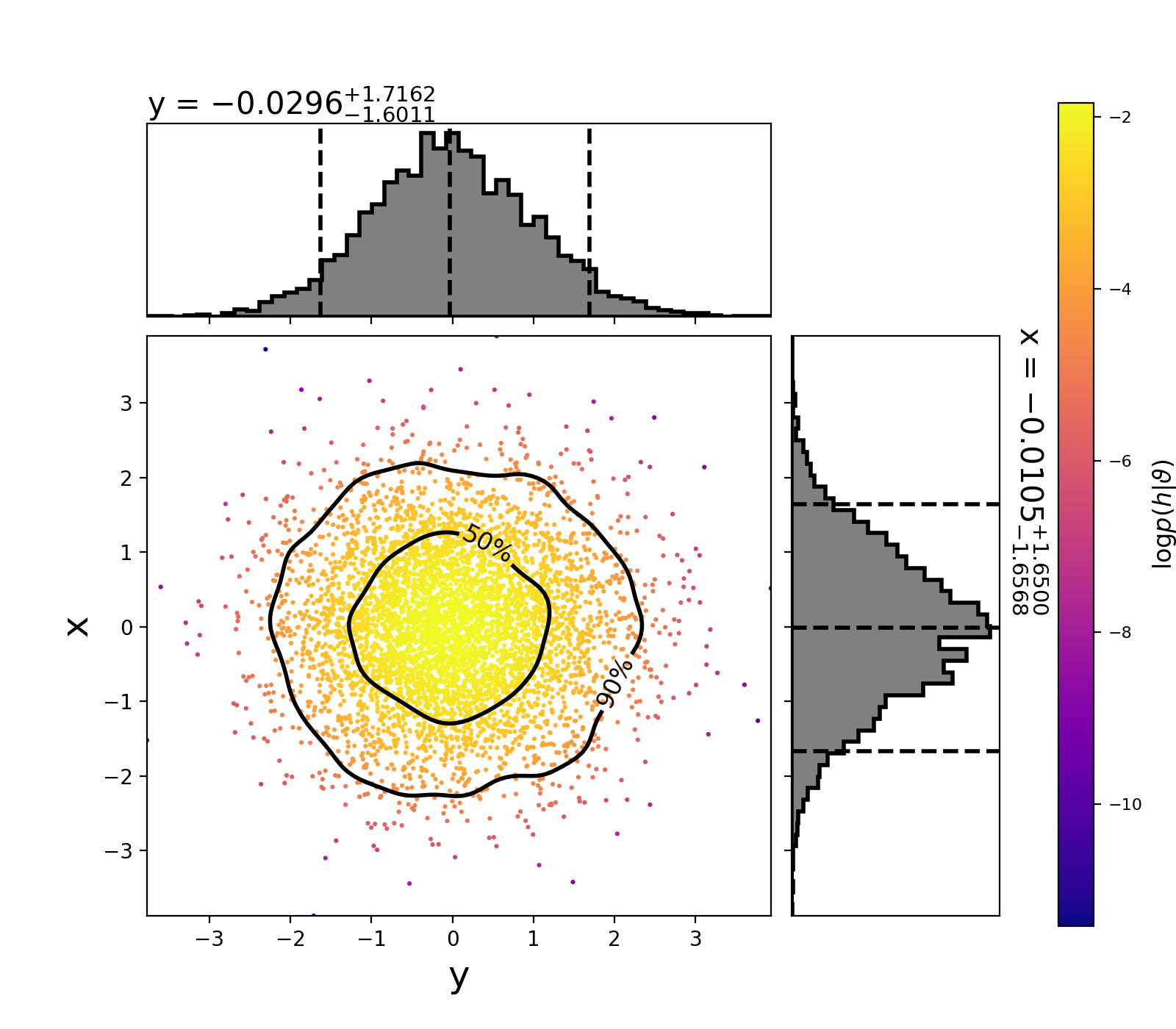
The scatter points show each walker’s position after the last iteration. The points are colored by the log likelihood at that point, with the 50th and 90th percentile contours drawn.
See below for more information about using pycbc_inference_plot_posterior.
To make a movie showing how the walkers evolved, run:
#!/bin/sh
pycbc_inference_plot_movie --verbose \
        --nprocesses 4 \
        --input-file normal2d.hdf \
        --output-prefix frames-normal2d \
        --movie-file normal2d_mcmc_evolution.mp4 \
        --cleanup \
        --plot-scatter \
        --plot-contours \
        --plot-marginal \
        --z-arg 'loglikelihood:$\log p(h|\vartheta)$' \
        --frame-step 1
Note
You need ffmpeg installed for the mp4 to be created.
See below for more information on using pycbc_inference_plot_movie.
Simulated BBH example
This example recovers the parameters of a simulated binary black-hole (BBH).
First, we need to create an injection.hdf file that specifies the
parameters of the simulated signal. To do that we will use
pycbc_create_injection. Like pycbc_inference,
pycbc_create_injections uses a configuration file to set the parameters of
the injections it will create. To create a binary-black hole with parameters
similar to GW150914, use the following configuration file:
[variable_params]

[static_params]
tc = 1126259462.420
mass1 = 37
mass2 = 32
ra = 2.2
dec = -1.25
inclincation = 2.5
coa_phase = 1.5
polarization = 1.75
distance = 100
f_ref = 20
f_lower = 18
approximant = IMRPhenomPv2
taper = start
Note the similarity to the configuration file for pycbc_inference: you must
have a [variable_params] section. If we wanted to randomize one or more
of the parameters, we would list them there, then add [prior] sections to
specify what distribution to draw the parameters from. In this case, however,
we want to fix the parameters, so we just put all of the necessary parameters
in the [static_params] section.
To create the injection file, run:
#!/bin/sh
pycbc_create_injections --verbose \
        --config-files injection.ini \
        --ninjections 1 \
        --seed 10 \
        --output-file injection.hdf \
        --variable-params-section variable_params \
        --static-params-section static_params \
        --dist-section prior
This will create the injection.hdf file, which we will give to
pycbc_inference. For more information on generating injection files, run
pycbc_create_injections --help.
Now we need to create the configuration file for pycbc_inference, calling
it inference.ini:
[model]
name = gaussian_noise
h1-low-frequency-cutoff = 20
l1-low-frequency-cutoff = 20

[sampler]
name = emcee_pt
nwalkers = 1000
ntemps = 4
effective-nsamples = 1000
checkpoint-interval = 2000
max-samples-per-chain = 1000

[sampler-burn_in]
burn-in-test = nacl & max_posterior

[variable_params]
; waveform parameters that will vary in MCMC
tc =
mass1 =
mass2 =
spin1_a =
spin1_azimuthal =
spin1_polar =
spin2_a =
spin2_azimuthal =
spin2_polar =
distance =
coa_phase =
inclination =
polarization =
ra =
dec =

[static_params]
; waveform parameters that will not change in MCMC
approximant = IMRPhenomPv2
f_lower = 18
f_ref = 20

[prior-tc]
; coalescence time prior
name = uniform
min-tc = 1126259462.32
max-tc = 1126259462.52

[prior-mass1]
name = uniform
min-mass1 = 10.
max-mass1 = 80.

[prior-mass2]
name = uniform
min-mass2 = 10.
max-mass2 = 80.

[prior-spin1_a]
name = uniform
min-spin1_a = 0.0
max-spin1_a = 0.99

[prior-spin1_polar+spin1_azimuthal]
name = uniform_solidangle
polar-angle = spin1_polar
azimuthal-angle = spin1_azimuthal

[prior-spin2_a]
name = uniform
min-spin2_a = 0.0
max-spin2_a = 0.99

[prior-spin2_polar+spin2_azimuthal]
name = uniform_solidangle
polar-angle = spin2_polar
azimuthal-angle = spin2_azimuthal

[prior-distance]
; following gives a uniform volume prior
name = uniform_radius
min-distance = 10
max-distance = 1000

[prior-coa_phase]
; coalescence phase prior
name = uniform_angle

[prior-inclination]
; inclination prior
name = sin_angle

[prior-ra+dec]
; sky position prior
name = uniform_sky

[prior-polarization]
; polarization prior
name = uniform_angle

;
;   Sampling transforms
;
[sampling_params]
; parameters on the left will be sampled in
; parametes on the right
mass1, mass2 : mchirp, q

[sampling_transforms-mchirp+q]
; inputs mass1, mass2
; outputs mchirp, q
name = mass1_mass2_to_mchirp_q
Here, we will use the emcee_pt sampler with 200 walkers and 20
temperatures. We will checkpoint (i.e., dump results to file) every 2000
iterations. Since we have provided an effective-nsamples argument and
a [sampler-burn_in] section, pycbc_inference will run until it has
acquired 1000 independent samples after burn-in, which is determined by the
nacl
test.
The number of independent samples is checked at each checkpoint: after dumping
the results, the burn-in test is applied and an autocorrelation length is
calculated. The number of independent samples is then
nwalkers x (the number of iterations since burn in)/ACL. If this number
exceeds effective-nsamples, pycbc_inference will finalize the results
and exit.
Now run:
#!/bin/sh
TRIGGER_TIME_INT=1126259462

# sampler parameters
CONFIG_PATH=inference.ini
OUTPUT_PATH=inference.hdf
SEGLEN=8
PSD_INVERSE_LENGTH=4
IFOS="H1 L1"
STRAIN="H1:aLIGOZeroDetHighPower L1:aLIGOZeroDetHighPower"
SAMPLE_RATE=2048
F_MIN=20
PROCESSING_SCHEME=cpu

# the following sets the number of cores to use; adjust as needed to
# your computer's capabilities
NPROCS=10

# start and end time of data to read in
GPS_START_TIME=$((TRIGGER_TIME_INT - SEGLEN))
GPS_END_TIME=$((TRIGGER_TIME_INT + SEGLEN))

# run sampler
# Running with OMP_NUM_THREADS=1 stops lalsimulation
# from spawning multiple jobs that would otherwise be used
# by pycbc_inference and cause a reduced runtime.
OMP_NUM_THREADS=1 \
pycbc_inference --verbose \
    --seed 12 \
    --instruments ${IFOS} \
    --gps-start-time ${GPS_START_TIME} \
    --gps-end-time ${GPS_END_TIME} \
    --psd-model ${STRAIN} \
    --psd-inverse-length ${PSD_INVERSE_LENGTH} \
    --fake-strain ${STRAIN} \
    --fake-strain-seed H1:44 L1:45 \
    --strain-high-pass ${F_MIN} \
    --sample-rate ${SAMPLE_RATE} \
    --data-conditioning-low-freq ${F_MIN} \
    --channel-name H1:FOOBAR L1:FOOBAR \
    --injection-file injection.hdf \
    --config-file ${CONFIG_PATH} \
    --output-file ${OUTPUT_PATH} \
    --processing-scheme ${PROCESSING_SCHEME} \
    --nprocesses ${NPROCS} \
    --force
Note that now we must provide for data. In this case, we are generating fake
Gaussian noise (via the fake-strain) module that is colored by the
advanced LIGO zero detuned high power PSD. We also have to provide arguments
for estimating a PSD.
The duration of data that will be analyzed is set by the
gps-(start|end)-time arguments. This data should be long enough such that
it encompasses the longest waveform admitted by our prior, plus our timing
uncertainty (which is determined by the prior on tc). Waveform duration is
approximately determined by the total mass of a system. The lowest total mass
(= mass1 + mass2) admitted by our prior is 20 solar masses. This corresponds
to a duration of approximately 6 seconds. (See the pycbc.waveform
module for utilities to estimate waveform duration.)
In addition, the beginning and end of the data segment will be corrupted by the
convolution of the inverse PSD with the data. To limit the amount of time that
is corrupted, we set --psd-inverse-length to 4. This limits the
corruption to at most the first and last four seconds of the data segment.
Combining these considerations, we end up creating 16 seconds of data: 8s for the waveform (we added a 2s safety buffer) + 4s at the beginning and end for inverse PSD corruption.
Since we are generating waveforms and analyzing a 15 dimensional parameter
space, this run will be much more computationally expensive than the analytic
example above. We recommend running this on a cluster or a computer with a
large number of cores. In the example, we have set the parallelization to use
10 cores. With these settings, it should checkpoint approximately every hour or
two. The run should complete in a few hours. If you would like to acquire more
samples, increase effective-nsamples.
GW150914 example
To run on GW150914, we can use the same configuration file as was used for the
BBH example, above.
(Download)
Now you need to obtain the real LIGO data containing GW150914. Do one of the following:
If you are a LIGO member and are running on a LIGO Data Grid cluster: you can use the LIGO data server to automatically obtain the frame files. Simply set the following environment variables:
export FRAMES="--frame-type H1:H1_HOFT_C02 L1:L1_HOFT_C02"
export CHANNELS="H1:H1:DCS-CALIB_STRAIN_C02 L1:L1:DCS-CALIB_STRAIN_C02"
If you are not a LIGO member, or are not running on a LIGO Data Grid cluster: you need to obtain the data from the Gravitational Wave Open Science Center. First run the following commands to download the needed frame files to your working directory:
wget https://www.gw-openscience.org/catalog/GWTC-1-confident/data/GW150914/H-H1_GWOSC_4KHZ_R1-1126257415-4096.gwf
wget https://www.gw-openscience.org/catalog/GWTC-1-confident/data/GW150914/L-L1_GWOSC_4KHZ_R1-1126257415-4096.gwf
Then set the following enviornment variables:
export FRAMES="--frame-files H1:H-H1_GWOSC_4KHZ_R1-1126257415-4096.gwf L1:L-L1_GWOSC_4KHZ_R1-1126257415-4096.gwf"
export CHANNELS="H1:GWOSC-4KHZ_R1_STRAIN L1:GWOSC-4KHZ_R1_STRAIN"
Now run:
#!/bin/sh
# trigger parameters
TRIGGER_TIME=1126259462.42

# data to use
# the longest waveform covered by the prior must fit in these times
SEARCH_BEFORE=6
SEARCH_AFTER=2

# use an extra number of seconds of data in addition to the data specified
PAD_DATA=8

# PSD estimation options
PSD_ESTIMATION="H1:median L1:median"
PSD_INVLEN=4
PSD_SEG_LEN=16
PSD_STRIDE=8
PSD_DATA_LEN=1024

# sampler parameters
CONFIG_PATH=inference.ini
OUTPUT_PATH=inference.hdf
IFOS="H1 L1"
SAMPLE_RATE=2048
F_HIGHPASS=15
F_MIN=20
PROCESSING_SCHEME=cpu

# the following sets the number of cores to use; adjust as needed to
# your computer's capabilities
NPROCS=10

# get coalescence time as an integer
TRIGGER_TIME_INT=${TRIGGER_TIME%.*}

# start and end time of data to read in
GPS_START_TIME=$((TRIGGER_TIME_INT - SEARCH_BEFORE - PSD_INVLEN))
GPS_END_TIME=$((TRIGGER_TIME_INT + SEARCH_AFTER + PSD_INVLEN))

# start and end time of data to read in for PSD estimation
PSD_START_TIME=$((TRIGGER_TIME_INT - PSD_DATA_LEN/2))
PSD_END_TIME=$((TRIGGER_TIME_INT + PSD_DATA_LEN/2))

# run sampler
# specifies the number of threads for OpenMP
# Running with OMP_NUM_THREADS=1 stops lalsimulation
# from spawning multiple jobs that would otherwise be used
# by inference and cause a reduced runtime.
OMP_NUM_THREADS=1 \
pycbc_inference --verbose \
    --seed 39392 \
    --instruments ${IFOS} \
    --gps-start-time ${GPS_START_TIME} \
    --gps-end-time ${GPS_END_TIME} \
    --channel-name ${CHANNELS} \
    ${FRAMES} \
    --strain-high-pass ${F_HIGHPASS} \
    --pad-data ${PAD_DATA} \
    --psd-estimation ${PSD_ESTIMATION} \
    --psd-start-time ${PSD_START_TIME} \
    --psd-end-time ${PSD_END_TIME} \
    --psd-segment-length ${PSD_SEG_LEN} \
    --psd-segment-stride ${PSD_STRIDE} \
    --psd-inverse-length ${PSD_INVLEN} \
    --sample-rate ${SAMPLE_RATE} \
    --data-conditioning-low-freq ${F_MIN} \
    --config-file ${CONFIG_PATH} \
    --output-file ${OUTPUT_PATH} \
    --processing-scheme ${PROCESSING_SCHEME} \
    --nprocesses ${NPROCS} \
    --force